数学物理学报, 2026, 46(5): 1913-1931

具有CTL免疫调控的病毒感染模型的稳定性与分支分析

宋晨玮,1, 徐瑞,2,*

1 晋中学院数学系 山西晋中 030619

2 山西大学复杂系统研究所 太原 030006

Stability and Bifurcation Analysis of a Virus Infection Model with CTL Immune Response

Song Chenwei,1, Xu Rui,2,*

1 Department of Mathematics, Jinzhong University, Shanxi Jinzhong, 030619

2 Complex Systems Research Center, Shanxi University, Taiyuan 030006

通讯作者: * 徐瑞, E-mail:xurui@sxu.edu.cn

收稿日期: 2025-09-15   修回日期: 2026-04-30  

基金资助: 国家自然科学基金(11871316)
国家自然科学基金(12501677)
山西省自然科学基金(202503021212261)
山西省高等学校科技创新项目(2025L117)

Received: 2025-09-15   Revised: 2026-04-30  

Fund supported: NSFC(11871316)
NSFC(12501677)
Natural Science Foundation of Shanxi Province(202503021212261)
Technological Innovation Programs of Higher Education Institutions in Shanxi Province(2025L117)

作者简介 About authors

宋晨玮,E-mail:scwei1014@163.com

摘要

该文基于细胞毒性T淋巴细胞(CTL)免疫应答机制和HIV 病毒感染的细胞内潜伏期, 建立了一个具有CTL 免疫反应和胞内时滞的HIV 感染动力学模型. 首先, 定义了两个关键阈值参数: 免疫失活再生数$\mathcal{R}_{0}$ 和免疫激活再生数$\mathcal{R}_{1}$. 其次, 在理论分析方面, 通过构造合适的Lyapunov 泛函, 证明了当$\mathcal{R}_{0}<1$ 时, 未感染平衡点是全局渐近稳定的. 进一步结合波动引理和Lyapunov 泛函方法, 建立了当$\mathcal{R}_{0}>1>\mathcal{R}_{1}$ 时, 免疫失活平衡点的全局渐近稳定性. 此外, 研究还发现, 当$\mathcal{R}_{1}>1$ 时, 系统在免疫激活平衡点附近展现出丰富的动力学特性: 无论是否引入胞内时滞, 模型均会出现Hopf 分支, 且在特定参数条件下可能出现更为复杂的双Hopf 分支. 最后, 在数值模拟部分, 针对无胞内时滞的情形, 通过规范性计算精确确定了分支方向、分支周期解的稳定性、振幅及周期等动力学性质; 对于存在胞内时滞的情形, 借助双参数分支分析验证了双Hopf 分支的存在性.

关键词: HIV 感染模型; CTL 免疫; 胞内时滞; 再生数; Hopf 分支

Abstract

Based on the immune response mechanism of cytotoxic T lymphocytes (CTL) and the intracellular latency of HIV infection, a dynamic model of HIV infection with CTL immune response and intracellular delay is established. Firstly, two key threshold parameters are defined: the immune inactivation reproduction number $\mathcal{R}_{0}$ and the immune activation reproduction number $ \mathcal{R}_{1}$. Second, in theoretical analysis, by constructing a suitable Lyapunov functional, it is proved that the uninfected equilibrium is globally asymptotically stable when $\mathcal{R}_{0}<1$. Further, by combining the wave lemma and Lyapunov functional method, the global asymptotic stability of the immune inactivation equilibrium is established when $\mathcal{R}_{0}>1>\mathcal{R}_{1}$. In addition, when $\mathcal{R}_{1}>1$, it is found that the system exhibits rich dynamic behaviors near the immune activation equilibrium: Hopf bifurcation will occur in the model regardless of the intracellular time delay, and even more complicated double Hopf bifurcation may occur. Numerical simulations quantitatively characterize the dynamical properties, employing normalization methods to precisely determine the bifurcation direction, stability of the periodic solutions, and their amplitude and period. In the presence of intracellular delay, a two-parameter bifurcation analysis rigorously establishes the existence of a double Hopf bifurcation.

Keywords: HIV infection model; CTL immunity; intracellular delay; reproduction number; Hopf bifurcation

PDF (937KB) 元数据 多维度评价 相关文章 导出 EndNote| Ris| Bibtex  收藏本文

本文引用格式

宋晨玮, 徐瑞. 具有CTL免疫调控的病毒感染模型的稳定性与分支分析[J]. 数学物理学报, 2026, 46(5): 1913-1931

Song Chenwei, Xu Rui. Stability and Bifurcation Analysis of a Virus Infection Model with CTL Immune Response[J]. Acta Mathematica Scientia, 2026, 46(5): 1913-1931

1 引言

人类免疫缺陷病毒1 型 (HIV-1) 是一种逆转录病毒, 能够特异性靶向攻击CD$4^{+}$辅助T细胞、巨噬细胞和树突状细胞等关键免疫细胞[1]. HIV-1 感染的临床进程呈现典型的阶段性特征: 在急性感染期, 病毒在宿主体内快速复制并广泛扩散; 随后进入临床潜伏期, 此阶段患者虽无明显临床症状, 但病毒仍在体内持续复制导致免疫系统遭受慢性损害; 最终发展为终末期, 此时病毒载量急剧上升, CD$4^{+}$T 细胞数量显著下降, 导致机体免疫功能严重受损, 形成获得性免疫缺陷综合征 (AIDS)[2,3]. 一旦病情进展至AIDS 阶段, 宿主的免疫系统便会全面崩溃, 丧失正常的免疫防御能力, 从而使得患者极易遭受各种病原体的侵袭, 引发各类严重的机会性感染和肿瘤, 严重威胁患者生命健康[4].

近年来, 多项研究揭示了CD$8^{+}$T 细胞介导的细胞毒性T淋巴细胞 (CTL) 免疫应答在病毒清除机制中的核心作用[5]. 实验研究表明, 随着CTL 免疫应答的增强, 宿主体内的病毒载量显著下降. 从免疫机制来看, CTL 介导的免疫记忆作为适应性免疫的关键特征, 可以从功能和细胞两个层面进行阐述: 在功能层面, 主要表现为宿主对特定病原体再次感染的保护性免疫能力; 在细胞层面, 则体现为病原体清除后抗原特异性免疫细胞数量的持续性维持. 这种免疫记忆机制不仅为理解抗病毒免疫提供了理论基础, 更为临床实现病毒感染的长期控制奠定了重要基础[6-8].

免疫记忆的建立主要依赖于CTL细胞群体的功能分化与协同作用. 研究表明, CTL 群体在免疫应答过程中会经历功能性分化, 形成两个具有不同生物学特性的的亚群: 效应性CTL (CTLe) 和记忆性前体CTL (CTLp). 其中, CTLe 能够直接识别并杀伤病毒感染细胞发挥抗病毒作用, 而CTLp 作为记忆性T 细胞的主要组成部分, 虽缺乏直接的效应功能, 却具有长期自我更新的特性[9,10]. 研究表明, 适度的抗原刺激对维持有效的免疫保护功能具有关键作用, 它不仅确保CTLe 的持续存在, 还促进了CTL 群体的动态平衡与更新. 这一机制使得机体在遭遇相同病原体再次感染时, 能够迅速启动有效的免疫防御应答. 具体而言, 病毒感染后, 细胞毒性T 淋巴细胞(CTL) 会分化为CTLp. 这类记忆性CTLp 构成了机体长期免疫记忆的核心组成部分. 值得注意的是, 记忆细胞群主要由CTLp 组成, 这些细胞表达能够特异性识别既往感染病毒的受体. 当机体再次遭遇相同病原体感染时, 这些记忆性CTLp 会迅速活化并分化为CTLe, 从而高效清除入侵的病毒, 发挥快速而强大的免疫保护作用[11,12]. 基于以上研究, Dominik 等在文献[13] 中建立了以下数学模型来分析CTL 免疫反应在病毒感染中的作用.

$\begin{equation}\label{1.1} \left\{ \begin{aligned} \dot x (t)&=s-d x(t)-\beta x(t) v(t),\\ \dot y (t)&=\beta x(t) v(t) -a y(t)-py(t)z(t),\\ \dot v (t)&=k y(t)-u v(t),\\ \dot w (t)&=c(1-q)y(t)w(t)-bw(t),\\ \dot z (t)&=cqy(t)w(t)-hz(t), \end{aligned} \right. \end{equation}$

其中, $x(t)$, $y(t)$, $v(t)$, $w(t)$$z(t)$ 分别表示$t$ 时刻未感染细胞、感染细胞、游离病毒、CTLp 和CTLe 的密度. 未感染细胞以恒定速率$s$ 产生, 并以自然死亡率$d$ 衰减. 病毒感染过程遵循质量作用定律, 感染率为$\beta xv$, 其中$\beta$ 为病毒感染率系数. 感染细胞以自然死亡率$a$ 死亡, 病毒在感染细胞内以$ky$ 的速率复制并释放, 游离病毒以速率$uv$ 被清除. 此外,CD8 细胞由两个亚群组成: CTLp 和CTLe. CTLp 在抗原刺激下以$c(1-q)yw$ 的速率增殖, 其中$c$ 为增殖系数, $q$ 为分化比例. 同时, CTLp 以$bw$ 的速率自然衰减, 并以$cqyw$ 的速率分化为CTLe. CTLe 则通过直接杀伤感染细胞发挥抗病毒作用, 并以$hz$ 的速率被清除.

系统(1.1) 采用双线性发生率$\beta xv$ 描述病毒-细胞的传播动力学, 该模型假设感染率与游离病毒浓度和未感染细胞数量的乘积成正比. 在感染初期, 游离病毒浓度远低于未感染细胞数量, 此时感染率近似与游离病毒浓度成正比, 双线性发生率是合理的. 然而, 随着感染进程的发展, 当病毒载量显著升高后, 由于靶细胞数量的限制和感染过程的饱和效应, 更合理的假设是感染率近似与未感染细胞的浓度成正比. 此外, 病毒进入靶细胞后需要经历逆转录形成病毒DNA, 随后在抗原刺激下转录为病毒RNA, 进而翻译成新的病毒蛋白, 最后组装成成熟病毒颗粒并从CD$4^{+}$T 细胞释放. 这一系列过程表明病毒感染后存在一个短暂的细胞内"隐蔽期", 在此期间细胞虽已被感染但尚未开始产生病毒[14].

基于文献[13,14]的研究成果, 考虑如下病毒感染动力学模型, 该模型通过引入胞内时滞来更准确地描述病毒复制的生物学过程. 其中, 参数$\tau$表示病毒感染细胞后完成逆转录、转录和翻译等步骤所需的平均时间, 即病毒复制的 "隐蔽期", 参数$m$ 是指不产生病毒的感染细胞的死亡率, $\mathrm{e}^{-m\tau}$ 描述从$t-\tau$$t$期间感染细胞存活的概率. 模型中的其他参数均与系统(1.1) 中保持相同的生物学意义.

$\begin{equation}\label{1.2} \left\{ \begin{aligned} \dot x (t)&=s-d x(t)-\frac{\beta x(t) v(t)}{ x(t)+v(t)},\\ \dot y (t)&=\frac{\beta \mathrm{e}^{-m\tau} x(t-\tau) v(t-\tau)}{ x(t-\tau)+v(t-\tau)}-a y(t)-py(t)z(t),\\ \dot v (t)&=k y(t)-u v(t),\\ \dot w (t)&=c(1-q)y(t)w(t)-bw(t),\\ \dot z (t)&=cqy(t)w(t)-hz(t), \end{aligned} \right. \end{equation}$

系统(1.2) 的初始条件

$\begin{equation}\label{1.3} \begin{aligned} x (\theta)=\phi_{1}(\theta),\quad &y (\theta)=\phi_{2}(\theta), \quad v (\theta)=\phi_{3}(\theta),\quad w(\theta)=\phi_{4}(\theta),\quad z(\theta)=\phi_{5}(\theta),\\ &\phi_{i}(\theta)\geq0,\quad\theta\in[-\tau,0),\quad\phi_{i}(0)>0\quad(i=1,2,3,4,5), \end{aligned} \end{equation}$

这里, 初值函数$\phi_{0}=(\phi_{1}(\theta),\phi_{2}(\theta),\phi_{3}(\theta),\phi_{4}(\theta),\phi_{5}(\theta))\in C([-\tau,0],\mathbb{R}_{+0}^{5})$, 其中$C([-\tau,0],\mathbb{R}_{+0}^{5})$ 表示从区间$[-\tau,0]$$\mathbb{R}_{+0}^{5}$ 的连续函数空间, $\mathbb{R}_{+0}^{5}=\{(x_{1},x_{2},x_{3},x_{4},x_{5}):x_{i}\geq0,i=1,2,3,4,5\}$.

2 解的正性和有界性

由泛函微分方程基本理论[15]可知, 系统 (1.2) 在初始条件(1.3)下存在唯一解$(x(t),y(t),v(t),w(t),z(t))$.

定理 2.1 系统(1.2) 满足初始条件(1.3) 的任一解在$[0,+\infty)$ 上有定义, 且恒为正.

$(x(t),y(t),v(t),w(t),z(t))$ 是系统(1.2) 满足初始条件(1.3) 的任一解. 首先证明$x(t)$ 的正性, 采用反证法, 假设存在$t_{1}>0$ 使得$x(t_{1})=0$$\mathrm{d}x(t_{1})/\mathrm{d}t\leq0$. 然而, 由系统(1.2) 的第一个方程可知$\mathrm{d}x(t_{1})/\mathrm{d}t>0$, 与假设矛盾. 因此, 对任意$t>0$, $x(t)>0$.

接下来, 证明对任意$t>0$, $y(t)>0$. 由系统(1.2) 的第二个方程可得

$\begin{equation}\label{2.1} \begin{aligned} y(t)=\left[\phi_{2}(0)+\int_{0}^{t}\left(\frac{\beta \mathrm{e}^{-m\tau }x(s-\tau)v(s-\tau)}{x(s-\tau)+v(s-\tau)}\right)\mathrm{e}^{(a+pz)s} \mathrm{d}s\right]\mathrm{e}^{\int_{0}^{t}-(a+pz(s))\mathrm{d}s}. \end{aligned} \end{equation}$

下面采用递推方法严格证明$y(t)$ 的正性. 首先, 当$t\in[0,\tau)$ 时, $v(t-\tau)=\phi_{3}(t-\tau)>0$, 由 (2.1) 式可得当$t\in[0,\tau)$ 时, 被积函数为正, 从而保证$y(t)>0$.$t\in[\tau,2\tau)$ 时, 通过相同的讨论可得$y(t)>0$. 进一步, 通过数学归纳法可得对任意$t>0$, 有$y(t)>0$.

由系统(1.2) 的第三和第四个方程可得

$\begin{equation}\label{2.2} \begin{aligned} &v(t)=\left(\phi_{3}(0)+k\int_{0}^{t}\mathrm{e}^{us}y(s)\mathrm{d}s\right)\mathrm{e}^{-ut},~ &w(t)=\phi_{4}(0)\mathrm{e}^{\int_{0}^{t}[c(1-q)y(s)-b]\mathrm{d}s}. \end{aligned} \end{equation}$

易证对任意的$t>0$,可得$v(t)>0$ 以及$w(t)>0$. 进一步由系统(1.2) 的第五个方程, 可得

$\begin{equation*} \begin{aligned} z(t)=\left[\phi_{5}(0)+cq{\int_{0}^{t}y(s)w(s)\mathrm{e}^{hs}\mathrm{d}s}\right]\mathrm{e}^{-ht}>0. \end{aligned} \end{equation*}$

基于上述分析, 系统(1.2) 的解$(x(t),y(t),v(t),w(t),z(t))$$t>0$ 时恒为正.

定理 2.2 系统(1.2) 满足初始条件(1.3) 的任一解最终有界.

$N(t)=x(t-\tau)+\mathrm{e}^{m\tau}y(t)$. 沿系统(1.2) 的正解计算$N(t)$ 的导数, 可得

$\begin{equation*} \begin{aligned} \dot{N}(t)&\leq s-\min\{a,d\}N(t), \end{aligned} \end{equation*}$

由比较定理可得

$\begin{equation*} \begin{aligned} \limsup_{t\rightarrow+\infty}N(t)\leq \frac{s}{\min\{a,d\}}.\\ \end{aligned} \end{equation*}$

进一步, 由系统(1.2) 的第三个方程可知

$\begin{equation*} \begin{aligned} \dot{v}(t)=ky(t)-uv(t)\leq\frac{ks\mathrm{e}^{-m\tau}}{\min\{a,d\}}-uv(t), \end{aligned} \end{equation*}$

求解可得$\limsup\limits_{t\rightarrow+\infty}v(t)\leq \frac{ks\mathrm{e}^{-m\tau}}{u\min\{a,d\}}$. 因此, $x(t),y(t)$$v(t)$ 是有界的. 结合$y(t)$ 的有界性, 进一步可得$w(t)$ 也是有界的.

下面证明$z(t)$ 的有界性, 易知$\phi_{5}(0)\mathrm{e}^{-ht}$ 有界, 对于解的另一部分$\mathrm{e}^{-ht}{\int_{0}^{t}cqy(s)w(s)\mathrm{e}^{hs}\mathrm{d}s}$, 利用洛必达法则可得

$\begin{equation*} \begin{aligned} \lim_{t\rightarrow\infty}\mathrm{e}^{-ht}\int_{0}^{t}cqy(s)w(s)\mathrm{e}^{hs}\mathrm{d}s \stackrel{H}{=}\lim_{t\rightarrow\infty}\frac{cqy(t)w(t)\mathrm{e}^{ht}}{\mathrm{e}^{ht}}=\frac{cqy(\infty)w(\infty)}{h}. \end{aligned} \end{equation*}$

$y(t)$$w(t)$ 的有界性可得$z(t)$ 也最终有界. 综上可得, 系统(1.2) 的任一解最终有界.

3 再生数和可行平衡点

显然, 系统(1.2) 总存在无病平衡点$E_{0}(s/d,0,0,0,0)$. 将系统(1.2) 的第二和第三个方程在$E_{0}$ 处线性化, 可得

$\begin{equation*} \begin{aligned} \frac{\mathrm{d}y (t)}{\mathrm{d}t}&=\beta \mathrm{e}^{-m\tau}v(t-\tau) -a y(t),\\ \frac{\mathrm{d}v (t)}{\mathrm{d}t}&=k y(t)-u v(t).\\ \end{aligned} \end{equation*}$

下面, 采用下一代矩阵法计算系统(1.2)的免疫失活再生数$\mathcal{R}_{0}$.

$\begin{equation*} \begin{aligned} \frac{\mathrm{d}X(t)}{\mathrm{d}t}=FX(t-\tau)-VX(t), \end{aligned} \end{equation*}$

其中

$\begin{gathered} X(t)= \left( \begin{array}{c} y(t)\\ v(t)\\ \end{array} \right), \end{gathered} \quad \begin{aligned} F=\begin{pmatrix} 0&\beta \mathrm{e}^{-m\tau}\\ 0 & 0\\ \end{pmatrix}, \quad V= \begin{pmatrix} a& 0\\ -k & u\\ \end{pmatrix}. \end{aligned} $

设初始感染分布为$\psi(0)=(\psi_{2},\psi_{3})$, 随着时间的推移, 时刻$t$ 的感染为$\psi(t)=\mathrm{e}^{-Vt}\psi(0)$.$0<t<\tau$ 时, 没有新的感染. 然而, 当$t>\tau$ 时, 时刻$t$ 的新感染率为 $F\psi(t-\tau)=F\mathrm{e}^{-V(t-\tau)}\psi(0)$. 因此, 新感染细胞数为

$\begin{align*} \int_{\tau}^{\infty}F\psi(t-\tau)\mathrm{d}t=\int_{\tau}^{\infty}F\mathrm{e}^{-V(t-\tau)}\psi(0)\mathrm{d}t=\int_{0}^{\infty}F\mathrm{e}^{-Vt}\psi(0)\mathrm{d}t=FV^{-1}\psi(0). \end{align*}$

由此可知, 系统(1.2) 的免疫失活再生数

$\begin{align*} \mathcal{R}_{0}=\rho(FV^{-1})=\frac{k\beta }{au}\mathrm{e}^{-m\tau}, \end{align*}$

这里$\rho(FV^{-1})$$FV^{-1}$ 的谱半径.

$\mathcal{R}_{0}>1$ 时, 除了无病平衡点, 系统(1.2) 存在免疫失活平衡点$E_{1}(x_{1},y_{1},v_{1},0,0)$, 其中

$\begin{equation*} \begin{aligned} x_{1}=\frac{ks}{au\mathrm{e}^{m\tau}(\mathcal{R}_{0}-1)+kd},\quad y_{1}=\frac{us(\mathcal{R}_{0}-1)}{u\mathrm{e}^{m\tau}(\mathcal{R}_{0}-1)+kd},\quad v_{1}=\frac{ks(\mathcal{R}_{0}-1)}{au\mathrm{e}^{m\tau}(\mathcal{R}_{0}-1)+kd}. \end{aligned} \end{equation*}$

进一步, 定义免疫激活再生数

$\mathcal{R}_{1}=\frac{[-(b \beta k+bdk-suc(1-q))+\sqrt{(b \beta k+bdk-suc(1-q))^{2}+4duc(1-q)skb}]}{2dbk}(\mathcal{R}_{0}-1).$

$\mathcal{R}_{1}>1$ 时, 除了$E_{0}$$E_{1}$, 系统(1.2) 存在免疫激活平衡点$E^{*}(x^{*},y^{*},v^{*},w^{*},z^{*})$, 其中

\begin{equation*} \begin{aligned} x^{*}&=\frac{-(b \beta k+bdk-suc(1-q))+\sqrt{(b \beta k+bdk-suc(1-q))^{2}+4duc(1-q)skb}}{2duc(1-q)},\\ y^{*}&=\frac{b}{c(1-q)},\quad v^{*}=\frac{kb}{uc(1-q)},\quad w^{*}=\frac{h(1-q)}{qb}z^{*}, \quad z^{*}={\frac{abk\left(\mathcal{R}_{1}-1\right)}{p \left(uc \left( 1-q \right)x^{*}+kb \right) }}. \end{aligned} \end{equation*}

4 阈值动力学

定理 4.1$\mathcal{R}_{0}<1$ 时, 系统(1.2) 的未感染平衡点$E_{0}$ 是局部渐近稳定的.

系统(1.2) 在未感染平衡点$E_{0}$ 处的特征方程为

$\begin{equation}\label{4.1} \begin{aligned} (\lambda+d)(\lambda+b)(\lambda+h)[\lambda^{2}+(a+u)\lambda+au(1-\mathcal{R}_{0})]=0. \end{aligned} \end{equation}$

显然, (4.1) 式有三个负实根$\lambda_{1}=-d,\lambda_{2}=-b,\lambda_{3}=-h$, 且(4.1) 式的其他根由下面的方程确定

$\begin{equation}\label{4.2} \begin{aligned} f_{1}(\lambda):=\lambda^{2}+(a+u)\lambda+au(1-\mathcal{R}_{0})=0. \end{aligned} \end{equation}$

$\mathcal{R}_{0}<1$ 时, 易得(4.1) 式的所有特征根都具有负实部, 未感染平衡点$E_{0}$ 局部渐近稳定. 当$\mathcal{R}_{0}>1$ 时, 可得$f(0)<0, f(+\infty)\rightarrow+\infty$, 由介值定理可得 (4.1) 式至少有一个正实根, 故未感染平衡点$E_{0}$ 不稳定.

定理 4.2$\mathcal{R}_{0}<1$ 时, 系统(1.2) 的未感染平衡点$E_{0}$ 是全局渐近稳定的.

$(x(t),y(t),v(t),w(t),z(t))$ 是系统(1.2) 满足初值条件(1.3) 的任一正解. 定义

$\begin{align*} W_{0}(t)=y(t)+\frac{a}{k}v(t)+\int_{t-\tau}^{t}\frac{\beta e^{-m\tau}x(u)v(u)}{x(u)+v(u)}\mathrm{d}u. \end{align*}$

沿系统(1.2) 的正解计算$W_{0}(t)$ 的导数, 可得

$\begin{align*} \dot{W}_{0}(t)=&\frac{\beta \mathrm{e}^{-m\tau} x(t) v(t)}{ x(t)+v(t)}-\frac{au}{k}v(t)-py(t)z(t)\\ =&-\frac{\beta \mathrm{e}^{-m\tau} v^{2}(t)}{ x(t)+v(t)}+\frac{au}{k}(\mathcal{R}_{0}-1)v(t)-py(t)z(t). \end{align*}$

因此, 当$\mathcal{R}_{0}<1$ 时, 可得$\dot{W}_{0}(t)\leq0$, 当且仅当$(x(t),y(t),v(t),w(t),z(t))=(s/d,0,0,0,0)$ 时等号成立. 进一步, 由定理4.1和LaSalle不变性原理可得, 未感染平衡点$E_{0}$ 是全局渐近稳定的.

定理 4.3$\mathcal{R}_{1}<1<\mathcal{R}_{0}$ 时, 系统(1.2) 的免疫失活平衡点$E_{1}$ 局部渐近稳定.

系统(1.2)在免疫失活平衡点$E_{1}$ 处的特征方程为

$\begin{equation}\label{4.3} \begin{aligned} (\lambda+b-c(1-q)y_{1})(\lambda+h)[\lambda^{3}+a_{11}(\tau)\lambda^{2}+a_{12}(\tau)\lambda+a_{13}(\tau)+(b_{11}(\tau)\lambda+b_{12}(\tau))\mathrm{e}^{-\lambda\tau}]=0, \end{aligned} \end{equation}$

这里

$\begin{equation*} \begin{aligned} a_{11}(\tau)&=a+u+d+\frac{\beta v_{1}^{2}}{(x_{1}+v_{1})^{2}},\quad a_{12}(\tau)=(a+u)\left(d+\frac{\beta v_{1}^{2}}{(x_{1}+v_{1})^{2}}\right)+au,\\ a_{13}(\tau)&=au\left(d+\frac{\beta v_{1}^{2}}{(x_{1}+v_{1})^{2}}\right),\quad b_{11}(\tau)=-\frac{k\beta x_{1}^{2}\mathrm{e}^{-m\tau}}{(x_{1}+v_{1})^{2}},\quad b_{12}(\tau)=-\frac{k\beta d x_{1}^{2}\mathrm{e}^{-m\tau}}{(x_{1}+v_{1})^{2}}. \end{aligned} \end{equation*}$

明显地, (4.3) 式存在负实根$\lambda_{1}=-b+c(1-q)y_{1},\lambda_{2}=-h$, (4.3) 的其他根由下面的方程决定

$\begin{equation}\label{4.4} \begin{aligned} f_{2}(\lambda):=\lambda^{3}+a_{11}(\tau)\lambda^{2}+a_{12}(\tau)\lambda+a_{13}(\tau)+(b_{11}(\tau)\lambda+b_{12}(\tau))\mathrm{e}^{-\lambda\tau}=0. \end{aligned} \end{equation}$

$\tau=0$ 时, (4.4) 式可改写为

$\begin{equation}\label{4.5} \begin{aligned} \lambda^{3}+a_{11}(0)\lambda^{2}+(a_{12}(0)+b_{11}(0))\lambda+(a_{13}(0)+b_{12}(0))=0, \end{aligned} \end{equation}$

这里

$\begin{equation*} \begin{aligned} &a_{11}(0)=a+u+d+\frac{\beta v_{1}^{2}}{(x_{1}+v_{1})^{2}},\\ &a_{12}(0)+b_{11}(0)=(a+u)\left(d+\frac{\beta v_{1}^{2}}{(x_{1}+v_{1})^{2}}\right)+au\left(1-\frac{1}{\mathcal{R}_{0}}\right),\\ &a_{13}(0)+b_{12}(0)=au\left(\frac{\beta v_{1}^{2}}{(x_{1}+v_{1})^{2}}+d\left(1-\frac{1}{\mathcal{R}_{0}}\right)\right). \end{aligned} \end{equation*}$

进一步计算可得

$\begin{equation*} \begin{aligned} &~a_{11}(0)(a_{12}(0)+b_{11}(0))-(a_{13}(0)+b_{12}(0))\\ =&\left(a+u+d+\frac{\beta v_{1}^{2}}{(x_{1}+v_{1})^{2}}\right)\left[(a+u)\left(d+\frac{\beta v_{1}^{2}}{(x_{1}+v_{1})^{2}}\right)+au\left(1-\frac{1}{\mathcal{R}_{0}}\right)\right]\\ &-au\left(\frac{\beta v_{1}^{2}}{(x_{1}+v_{1})^{2}}+d\left(1-\frac{1}{\mathcal{R}_{0}}\right)\right). \end{aligned} \end{equation*}$

$\mathcal{R}_{0}>1$ 时, 容易验证$a_{12}(0)+b_{11}(0)>0,a_{13}(0)+b_{12}(0)>0$$a_{11}(0)(a_{12}(0)+b_{11}(0))>a_{13}(0)+b_{12}(0)$. 因此, 根据Routh-Hurwitz 判据, 平衡点$E_{1}$ 是局部渐近稳定的.

$\tau>0$ 时, 令$\lambda=\mathrm{i}\omega (\omega>0)$ 是(4.4) 式的一对纯虚根. 将$\mathrm{i}\omega (\omega>0)$ 代入(4.4), 分离实虚部可得

$\begin{equation}\label{4.6} \begin{aligned} -\omega^{3}+a_{12}(\tau)\omega&=-b_{11}(\tau)\omega\cos\omega\tau+b_{12}(\tau)\sin\omega\tau,\\ -a_{11}(\tau)\omega^{2}+a_{13}(\tau)&=-b_{11}(\tau)\omega\sin\omega\tau-b_{12}(\tau)\cos\omega\tau. \end{aligned} \end{equation}$

将(4.6) 式两边平方且相加可得

$\begin{equation}\label{4.7} \begin{aligned} \omega^{6}+(a_{11}^{2}(\tau)-2a_{12}(\tau))\omega^{4}+(a_{12}^{2}(\tau)-2a_{11}(\tau)a_{13}(\tau)-b_{11}^{2}(\tau))\omega^{2}+(a_{13}^{2}(\tau)-b_{12}^{2}(\tau))=0, \end{aligned} \end{equation}$

这里

$\begin{equation*} \begin{aligned} &a_{11}^{2}(\tau)-2a_{12}(\tau)=a^{2}+u^{2}+\left(d+\frac{\beta v_{1}^{2}}{(x_{1}+v_{1})^{2}}\right)^{2},\\ &a_{12}^{2}(\tau)-2a_{11}(\tau)a_{13}(\tau)-b_{11}^{2}(\tau)=(a^{2}+u^{2})\left(d+\frac{\beta v_{1}^{2}}{(x_{1}+v_{1})^{2}}\right)^{2}+a^{2}u^{2}\left(1-\frac{1}{\mathcal{R}_{0}^{2}}\right),\\ &a_{13}^{2}(\tau)-b_{12}^{2}(\tau)=a^{2}u^{2}\left(2d+\frac{\beta v_{1}^{2}}{(x_{1}+v_{1})^{2}}\right)\frac{\beta v_{1}^{2}}{(x_{1}+v_{1})^{2}}+a^{2}u^{2}d^{2}\left(1-\frac{1}{\mathcal{R}_{0}^{2}}\right). \end{aligned} \end{equation*}$

进一步计算可得

$\begin{equation*} \begin{aligned} &~~~(a_{11}^{2}(\tau)-2a_{12}(\tau))(a_{12}^{2}(\tau)-2a_{11}(\tau)a_{13}(\tau)-b_{11}^{2}(\tau))-(a_{13}^{2}(\tau)-b_{12}^{2}(\tau))\\ &=a^{2}u^{2}\left[a^{2}+u^{2}+\left(2d+\frac{\beta v_{1}^{2}}{(x_{1}+v_{1})^{2}}\right)\frac{\beta v_{1}^{2}}{(x_{1}+v_{1})^{2}}\right]\left(1-\frac{1}{\mathcal{R}_{0}^{2}}\right)\\ &~~~+(a^{4}+a^{2}u^{2}+u^{4})\left(d+\frac{\beta v_{1}^{2}}{(x_{1}+v_{1})^{2}}\right)^{2} +a^{2}u^{2}d^{2}>0. \end{aligned} \end{equation*}$

同样可由Routh-Hurwitz 判据可知, (4.7) 式无正实根. 因此, 对任意$\tau\geq0$, 特征方程 (4.4) 的所有根均具有负实部,故平衡点$E_{1}$ 局部渐近稳定.

定理 4.4$\mathcal{R}_{1}<1<\mathcal{R}_{0}$ 时, 系统(1.2) 的免疫失活平衡点$E_{1}$ 是全局渐近稳定的.

$(x(t),y(t),v(t),w(t),z(t))$ 是系统(1.2) 满足初值条件(1.3) 的任意解. 定义

$\begin{align*} W_{1}(t)=&\left(x(t)-x_{1}-\int_{x_{1}}^{x(t)}\frac{x_{1}(u+v_{1})}{(x_{1}+v_{1})u}\mathrm{d}u\right)+\mathrm{e}^{m\tau}\left(y(t)-y_{1}-y_{1}\ln\frac{y(t)}{y_{1}}\right)\\ &+\frac{a}{k}\left(v(t)-v_{1}-v_{1}\ln\frac{v(t)}{v_{1}}\right)+m(w(t)+z(t))\\ &+\beta\int_{t-\tau}^{t}\left[\frac{x(u)v(u)}{x(u)+v(u)}-\frac{x_{1}v_{1}}{x_{1}+v_{1}}-\frac{x_{1}v_{1}}{x_{1}+v_{1}}\ln\frac{(x_{1}+v_{1})x(u)v(u)}{x_{1}v_{1}(x(u)+v(u))}\right]\mathrm{d}u, \end{align*}$

沿系统(1.2) 的正解计算$W_{1}(t)$ 的导数, 可得

$\begin{align*} \frac{\mathrm{d}W_{1}}{\mathrm{d}t} =&-\frac{d(x(t)-v_{1})^{2}}{(x_{1}+v_{1})x(t)}-\frac{\beta x_{1}v_{1}}{x_{1}+v_{1}}\left[\frac{x_{1}(x(t)+v_{1})}{(x_{1}+v_{1})x(t)}-1-\ln\frac{x_{1}(x(t)+v_{1})}{(x_{1}+v_{1})x(t)}\right]\\ &-\frac{\beta x_{1}v_{1}}{x_{1}+v_{1}}\left[\frac{x(t-\tau) v(t-\tau)y_{1}(x_{1}+v_{1})}{x(t-\tau)+v(t-\tau)x_{1}v_{1}y(t)}-1-\ln\frac{x(t-\tau) v(t-\tau)y_{1}(x_{1}+v_{1})}{x(t-\tau)+v(t-\tau)x_{1}v_{1}y(t)}\right]\\ &-\frac{\beta x_{1}v_{1}}{x_{1}+v_{1}}\left[\frac{x(t)+v(t)}{x(t)+v_{1}}-1-\ln\frac{x(t)+v(t)}{x(t)+v_{1}}\right]-\frac{\beta x_{1}v_{1}}{x_{1}+v_{1}}\left[\frac{y(t)}{y_{1}}\frac{v_{1}}{v(t)}-1-\ln\frac{y(t)}{y_{1}}\frac{v_{1}}{v(t)}\right]\\ &-\frac{\beta x_{1}x(t)(v(t)-v_{1})^{2}}{(x_{1}+v_{1})(x(t)+v_{1})(x(t)+v(t))}-[mh+p(y(t)-y_{1})]z(t)\mathrm{e}^{m\tau}\\&+mc\left(y(t)-\frac{b}{c}\right)w(t). \end{align*}$

假设初始条件满足$y(0)>y_{1}$, 可以选取足够小的$m>0$ 使得 $\dot{W_{1}}(t)<0$. 这一性质表明解轨迹将在有限时间$T_{1}>0$ 内进入区域 $y(t)<y_{1}+\varepsilon$, 并在随后始终保持在这个区域内. 反之, 若初始条件满足$y(0)<y_{1}$, 同样可选取合适的$m>0$ 使得 $\dot{W_{1}}(t)<0$, 此时解轨迹将始终在区域 $y(t)<y_{1}+\varepsilon$ 内. 进一步, 由已知条件

$\frac{b}{c(1-q)}-y_{1}>0,$

可知通过选择适当的$m$ 可确保$\frac{b}{c(1-q)}>y_{1}>y-\varepsilon$. 因此, 存在某个有限时刻$T>T_{1}$ 使得解进入$y\leq\frac{b}{c(1-q)}$ 的区域, 并在 $t\in[T,\infty)$ 期间停留在这个区域.

接下来证明解轨线渐近趋近于平衡点$E_{1}$. 定义$f_{\infty}=\liminf\limits_{t\rightarrow\infty}f(t),\quad f^{\infty}=\limsup\limits_{t\rightarrow\infty}f(t).$ 根据波动引理, 存在时间序列$t_{n}$ 满足当$n\rightarrow\infty$ 时, $t_{n}\rightarrow\infty$, 且 $\lim\limits_{n\rightarrow\infty}w(t_{n})=w^{\infty},\quad \lim\limits_{n\rightarrow\infty}\dot{w}(t_{n})=0.$ 假设$t=t_{n}$, 由系统的第四个方程可得 $\dot w (t_{n})=c(1-q)y(t_{n})w(t_{n})-bw(t_{n}).$$n\rightarrow\infty$ 时, 可得 $c(1-q)y^{\infty}w^{\infty}\geq bw^{\infty}.$由于$y(t)\leq\frac{b}{c(1-q)}$, 上式仅在$w^{\infty}=0$ 成立. 这表明系统(1.2) 的渐近行为可由以下系统描述

$\begin{equation}\label{4.8} \left\{ \begin{aligned} \dot x (t)&=s-d x(t)-\frac{\beta x(t) v(t)}{ x(t)+v(t)},\\ \dot y (t)&=\frac{\beta \mathrm{e}^{-m\tau} x(t-\tau) v(t-\tau)}{ x(t-\tau)+v(t-\tau)}-a y(t),\\ \dot v (t)&=k y(t)-u v(t). \end{aligned} \right. \end{equation}$

系统(4.8) 具有两个平衡点$\tilde{E}_{0}(s/d,0,0)$$\tilde{E}_{1}(x_{1},y_{1},v_{1})$. 稳定性分析表明, 当$\mathcal{R}_{1}<1<\mathcal{R}_{0}$ 时, $\tilde{E}_{0}$ 不稳定, 而$\tilde{E}_{1}$ 局部渐近稳定. 进一步, 对子系统(4.8) 应用Lyapunov 稳定性定理可证得: 当$\mathcal{R}_{1}<1<\mathcal{R}_{0}$ 时, 子系统(4.8) 的平衡点 $\tilde{E}_{1}$ 全局渐近稳定, 进一步原系统(1.2) 对应的平衡点$E_{1}$ 同样具有全局渐近稳定性.

下面, 我们研究免疫激活平衡点$E^{*}$ 的稳定性. 系统(1.2) 在平衡点$E^{*}$ 处的特征方程为

$\begin{equation}\label{4.9} \begin{aligned} &~\lambda^{5}+c_{21}(\tau)\lambda^{4}+c_{22}(\tau)\lambda^{3}+c_{23}(\tau)\lambda^{2} +c_{24}(\tau)\lambda+c_{25}(\tau)\\ &+(c_{11}(\tau)\lambda^{3}+c_{12}(\tau)\lambda^{2}+c_{13}(\tau)\lambda)\mathrm{e}^{-\lambda\tau}=0, \end{aligned} \end{equation}$

这里

$\begin{align*} c_{21}(\tau)=&d+\frac {\beta v^{*2}}{(x^{*}+v^{*}) ^{2}}+h+pz^{*}+a+u,\\ c_{22}(\tau)=&\left(d+\frac {\beta v^{*2}}{(x^{*}+v^{*}) ^{2}}\right)(h+pz^{*}+a+u)+h(pz^{*}+a+u)+(pz^{*}+a)u+phz^{*},\\ c_{23}(\tau)=&\left(d+\frac {\beta v^{*2}}{(x^{*}+v^{*}) ^{2}}\right)h(pz^{*}+a+u)+\left(d+\frac {\beta v^{*2}}{(x^{*}+v^{*})^{2}}\right)(pz^{*}+a)u+h(pz^{*}+a)u\\ &+phz^{*}\left(d+\frac {\beta v^{2}}{ (x^{*}+v^{*}) ^{2}}+u+b\right),\\ c_{24}(\tau)=&\left(d+\frac {\beta v^{*2}}{(x^{*}+v^{*}) ^{2}}\right)h(pz^{*}+a)u+phz^{*}\left(d+\frac {\beta v^{*2}}{ (x^{*}+v^{*})^{2}}\right)(b+u)+phz^{*}ub,\\ c_{25}(\tau)=&phz^{*}\left(d+\frac {\beta v^{*2}}{ (x^{*}+v^{*})^{2}}\right)ub,\\ c_{11}(\tau)=&-\frac{k\beta x^{*2}\mathrm{e}^{-m\tau}}{ (x^{*}+v^{*}) ^{2}},\\ c_{12}(\tau)=&-\frac{k\beta x^{*2}\mathrm{e}^{-m\tau}}{ (x^{*}+v^{*}) ^{2}}(d+h),\\ c_{13}(\tau)=&-\frac{k\beta x^{*2}\mathrm{e}^{-m\tau}}{ (x^{*}+v^{*})^{2}}dh. \end{align*}$

$\tau=0$ 时, 特征方程(4.9) 简化为如下五次多项式

$\begin{equation}\label{4.10} \begin{aligned} \lambda^{5}+b_{1}\lambda^{4}+b_{2}\lambda^{3}+b_{3}\lambda^{2}+b_{4}\lambda+b_{5}=0, \end{aligned} \end{equation}$

其中

$\begin{align*} b_{1}=&d+\frac {\beta v^{*2}}{(x^{*}+v^{*}) ^{2}}+h+pz^{*}+a+u,\\ b_{2}=&\left(d+\frac {\beta v^{*2}}{(x^{*}+v^{*})^{2}}\right)(h+pz^{*}+a+u)+h(pz^{*}+a+u)+phz^{*}+\frac{k\beta x^{*}v^{*}}{ (x^{*}+v^{*}) ^{2}},\\ b_{3}=&\left(d+\frac {\beta v^{*2}}{(x^{*}+v^{*}) ^{2}}\right)h(pz^{*}+a+u)+\frac {\beta v^{*2}}{(x^{*}+v^{*}) ^{2}}(pz^{*}+a)u+phz\left(d+\frac {\beta v^{*2}}{ (x^{*}+v^{*}) ^{2}}+u+b\right)\\ &+\frac{k\beta x^{*}v^{*}}{ (x^{*}+v^{*}) ^{2}}(d+h),\\ b_{4} =&\frac {\beta v^{*2}}{(x^{*}+v^{*}) ^{2}}h(pz^{*}+a)u+phz^{*}\left(d+\frac {\beta v^{*2}}{ (x^{*}+v^{*})^{2}}\right)(b+u)+phz^{*}ub+\frac{k\beta x^{*}v^{*}}{ (x^{*}+v^{*})^{2}}dh,\\ b_{5}=&phz^{*}\left(d+\frac {\beta v^{*2}}{ (x^{*}+v^{*})^{2}}\right)ub. \end{align*}$

基于特征方程的系数, 构造如下Routh-Hurwitz行列式序列

$\begin{align*} \Delta_{1}=&b_{1}>0,\quad \quad \Delta_{2}=b_{1}b_{2}-b_{3},\quad \Delta_{3}=b_{3}(b_{1}b_{2}-b_{3})-b_{1}(b_{1}b_{4}-b_{5}),\\ \Delta_{4}=&b_{4}\Delta_{3}+b_{5}[(b_{1}b_{4}-b_{5})-b_{2}(b_{1}b_{2}-b_{3})],\quad\quad \Delta_{5}=b_{5}\Delta_{4}. \end{align*}$

根据Routh-Hurwitz 稳定性判据, 平衡点$E^{*}$的局部稳定性由上述行列式的符号决定: 当且仅当 行列式满足$\Delta_{i}>0(i=1\cdots5)$ 时, 平衡点$E^{*}$ 是局部渐近稳定的; 反之, 该平衡点 $E^{*}$ 是不稳定的.

引理 4.1 假设$\Delta_{2},\Delta_{3}$$\Delta_{4}$ 的符号随参数变化由正转负, 则满足以下规律

${\bf (i)}$$\Delta_{3}$ 的符号变化先于$\Delta_{2}$; ${\bf (ii)}$$\Delta_{4}$ 的符号变化先于$\Delta_{3}$.

首先证明$\Delta_{3}$ 的符号变化先于$\Delta_{2}$.$\Delta_{3}=0$, 则$\Delta_{2}$ 可表示为 $\Delta_{2}=\frac{b_{1}(b_{1}b_{4}-b_{5})}{b_{3}}.$ 通过直接计算可得

$\begin{align*} b_{1}b_{4}-b_{5}=&\left(\frac {\beta v^{*2}}{(x^{*}+v^{*}) ^{2}}h(pz^{*}+a)u+\frac{k\beta x^{*}v^{*}}{ ( x^{*}+v^{*}) ^{2}}dh+phz^{*}\left(d+\frac {\beta v^{*2}}{ ( x^{*}+v^{*}) ^{2}}\right)(b+u)\right)\\ &\times\left(d+\frac {\beta v^{*2}}{(x+v) ^{2}}+h+pz^{*}+a+u\right)+(h+pz^{*}+a+u)phz^{*}ub>0. \end{align*}$

由此可得$\Delta_{2}>0$. 进一步, 当$\Delta_{2}=0$ 时, 有$\Delta_{3}=-b_{1}(b_{1}b_{4}-b_{5})<0.$ 上述结果表明,$\Delta_{3}$ 的符号变化先于$\Delta_{2}$.

下面证明$\Delta_{4}$ 的符号变化先于$\Delta_{3}$.$\Delta_{3}=0$ 时, 有$b_{1}b_{4}-b_{5}=\frac{b_{3}\Delta_{2}}{b_{1}}.$ 将其代入$\Delta_{4}$ 的表达式, 可得

$\Delta_{4}=b_{5}[(b_{1}b_{4}-b_{5})-b_{2}\Delta_{2}]=-\frac{b_{5}}{b_{1}}\Delta_{2}^{2}<0.$

反之, 当$\Delta_{4}=0$ 时, 有$\Delta_{3}=\frac{b_{5}}{b_{4}}[b_{2}\Delta_{2}-(b_{1}b_{4}-b_{5})].$ 结合关系式$b_{1}b_{4}-b_{5}=\frac{1}{b_{1}}[b_{3}\Delta_{2}-\Delta_{3}]$, 最终可得

$\Delta_{3}=\frac{b_{5}\Delta_{2}^{2}}{b_{1}b_{4}-b_{5}}>0.$

上述讨论结果表明, 当$\Delta_{4}$ 的符号从正到负穿过零时, $E^{*}$ 失去稳定性的唯一可能是Hopf 分支的出现. 根据文献[定理 2] 可得, 若存在参数值$h^{*}$ 使得$\Delta_{4}(h^{*})=0$, 则特征方程 (4.9) 存在一对纯虚根, 且其余所有根均具有负实部.

为确定Hopf分支方向, 不失一般性, 设$\lambda=\rm{i}\omega (\omega > 0)$$(4.9)$ 式的一对纯虚根,将$\rm{i}\omega (\omega > 0)$ 代入$(4.9)$ 式, 分离实虚部可得

$\begin{align*} -\omega^{4}+b_{2}\omega^{2}=b_{4},\quad \quad -b_{1}\omega^{4}+b_{3}\omega^{2}=b_{5}. \end{align*}$

对特征方程(4.9) 关于参数$h$ 求导, 可得

$\begin{align*} \frac{\mathrm{d}\lambda}{\mathrm{d}h}=-\frac{1}{2}\frac{\frac{\mathrm{d}b_{1}}{\mathrm{d}h}\omega^{4}-\frac{\mathrm{d}b_{3}}{\mathrm{d}h}\omega^{2}+\frac{\mathrm{d}b_{5}}{\mathrm{d}h}-(\frac{\mathrm{d}b_{2}}{\mathrm{d}h}\omega^{3}-\frac{\mathrm{d}b_{4}}{\mathrm{d}h}\omega)\mathrm{i}}{2\omega^{4}-b_{2}\omega^{2}-(2b_{1}\omega^{3}-b_{3}\omega)\mathrm{i}}. \end{align*}$

由此可进一步推得

$\begin{align*} \frac{\mathrm{d}(\mathrm{Re}\lambda)}{\mathrm{d}h}=-\frac{1}{2}\frac{\Delta_{2}}{(2\omega^{3}-b_{2}\omega)^{2}+(2b_{1}\omega^{2}-b_{3})^{2}}\frac{\mathrm{d}\Delta_{4}}{\mathrm{d}h}. \end{align*}$

定理 4.5$\mathcal{R}_{1}>1$$\tau=0$ 时, 对系统(1.2), 有

${\bf(i)}$ 若所有$\Delta_{i}>0~(i=1\cdots5)$, 则平衡点$E^{*}$ 是局部渐近稳定的;

${\bf(ii)}$ 若存在正零点$h^{*}$ 使得$\Delta_{4}(h)=0$$\Delta_{4}'(h^{*})\neq0$, 则系统在$h=h^{*}$ 处出现Hopf分支.

$\tau>0$ 时, 不失一般性, 假设$\lambda=\mathrm{i}\omega(\omega>0)$ 是 (4.9) 式的一对纯虚根. 将$\lambda=\mathrm{i}\omega$ 代入 (4.9) 式, 分离实虚部可得

$\begin{equation}\label{4.11} \begin{split} \omega^{5}-c_{22}(\tau)\omega^{3}+c_{24}(\tau)\omega=&(c_{11}(\tau)\omega^{3}-c_{13}(\tau)\omega)\cos(\omega\tau)-c_{12}(\tau)\omega^{2}\sin(\omega\tau),\\ c_{21}(\tau)\omega^{4}-c_{23}(\tau)\omega^{2}+c_{25}(\tau)=&(c_{11}(\tau)\omega^{3}-c_{13}(\tau)\omega)\sin(\omega\tau)+c_{12}(\tau)\omega^{2}\cos(\omega\tau). \end{split} \end{equation}$

将上述两式分别平方后相加, 可得

$\begin{equation}\label{4.12} \begin{aligned} \omega^{10}+c_{1}(\tau)\omega^{8}+c_{2}(\tau)\omega^{6}+c_{3}(\tau)\omega^{4}+c_{4}(\tau)\omega^{2}+c_{5}(\tau)=0, \end{aligned} \end{equation}$

其中系数定义为

$\begin{align*} c_{1}(\tau)&=c_{21}^{2}(\tau)-2c_{22}(\tau)>0,\\ c_{2}(\tau)&=c_{22}^{2}(\tau)+2c_{24}(\tau)-2c_{21}(\tau)c_{23}(\tau)-c_{11}^{2}(\tau),\\ c_{3}(\tau)&=c_{23}^{2}(\tau)-2c_{22}(\tau)c_{24}(\tau)+2c_{21}(\tau)c_{25}(\tau)+2c_{11}(\tau)c_{13}(\tau)-c_{12}^{2}(\tau),\\ c_{4}(\tau)&=c_{24}^{2}(\tau)-2c_{23}(\tau)c_{25}(\tau)-c_{13}^{2}(\tau),\\ c_{5}(\tau)&=c_{25}^{2}(\tau)>0. \end{align*}$

$z=\omega^{2}$, 则(4.12) 式可改写为

$\begin{equation}\label{4.13} \begin{aligned} z^{5}+c_{1}(\tau)z^{4}+c_{2}(\tau)z^{3}+c_{3}(\tau)z^{2}+c_{4}(\tau)z+c_{5}(\tau)=0. \end{aligned} \end{equation}$

引理 4.2 基于笛卡尔符号法则, 方程(4.13)的根具有如下性质

${\bf (i)}$ 当$c_{2}(\tau)>0$, $c_{3}(\tau)>0$, $c_{4}(\tau)>0$ 时, 方程(4.13) 无正实根;

${\bf(ii)}$ 如果下面条件中的一个被满足

$c_{2}(\tau)>0$, $c_{3}(\tau)<0$$c_{4}(\tau)>0$,

$c_{2}(\tau)>0$, $c_{3}(\tau)<0$$c_{4}(\tau)<0$,

$c_{2}(\tau)>0$, $c_{3}(\tau)>0$$c_{4}(\tau)<0$,

$c_{2}(\tau)<0$, $c_{3}(\tau)>0$$c_{4}(\tau)>0$,

$c_{2}(\tau)<0$, $c_{3}(\tau)>0$$c_{4}(\tau)<0$,

$c_{2}(\tau)<0$, $c_{3}(\tau)<0$$c_{4}(\tau)<0$,

方程(4.13) 可能有两个正实根或无正实根;

${\bf(iii)}$ 当$c_{2}(\tau)<0$, $c_{3}(\tau)>0$$c_{4}(\tau)<0$ 时, 方程(4.13) 可能有两个或四个正实根.

若方程(4.13) 不存在正实根, 即$\omega=\sqrt{z}$ 不存在, 则临界分支参数$\tau$ 不存在. 此时, 系统在平衡点 $E^{*}$ 不会发生Hopf 分支, 其稳定性保持不变.

下面, 考虑方程(4.13) 具有两个不同正实根$z_{j}(j=1,2)$ 的情形, 则$\omega_{j}=\sqrt{z_{j}}(j=1,2)$ 即为方程(4.12) 的正根, 且满足$\omega_{1}>\omega_{2}$. 由 (4.11) 式可得

$\begin{equation}\label{4.14} \left\{ \begin{split} \sin(\omega_{j}\tau)&=\frac{A(\omega_{j}\tau)B(\omega_{j}\tau)-C(\omega_{j}\tau)D(\omega_{j}\tau)}{A^{2}(\omega_{j}\tau)+D^{2}(\omega_{j}\tau)},\\ \cos(\omega_{j}\tau)&=\frac{B(\omega_{j}\tau)D(\omega_{j}\tau)+A(\omega_{j}\tau)C(\omega_{j}\tau)}{A^{2}(\omega_{j}\tau)+D^{2}(\omega_{j}\tau)}, \end{split} \right. \end{equation}$

其中

$\begin{align*} A(\omega_{j}\tau)&=c_{11}(\tau)\omega_{j}^{3}-c_{13}(\tau)\omega_{j},\\ B(\omega_{j}\tau)&=c_{21}(\tau)\omega_{j}^{4}-c_{23}(\tau)\omega_{j}^{2} +c_{25}(\tau),\\ C(\omega_{j}\tau)&=\omega_{j}^{5}-c_{22}(\tau)\omega_{j}^{3}+c_{24}(\tau)\omega_{j},\\ D(\omega_{j}\tau)&=c_{12}\omega_{j}^{2}. \end{align*}$

定义$\theta_{j}\in[0,2\pi]$, 使得$\sin(\theta_{j})$, $\cos(\theta_{j})$ 分别由(4.14) 式的右侧给出. 由此可得

$\omega_{j}\tau_{n}^{j}=\theta_{j}(\tau_{n}^{j})+2\pi n,\quad j=1,2,n=0,1,2,\cdots$

定义映射

$\begin{equation*} \begin{split} S_{nj}(\tau_{n}^{j})=\tau_{n}^{j}-\frac{\theta_{j}(\tau_{n}^{j})+2\pi n}{\omega_{j}}, \quad n\in N, \tau\in(0,\tau_{\max}). \end{split} \end{equation*}$

$\pm \rm{i}w_{j}(\tau^{*})$ 是特征方程(4.12) 的纯虚根当且仅当 $\tau^{*}$$S_{n}(\tau)$ 的零点. 根据文献[17,定理 2.2], 可得以下Hopf 分支判据

定理 4.6 对任意$n\in N$, $j=1,2$, 当$S_{nj}(\tau^{*})=0$ 时, 特征方程 (4.12) 存在一对单纯虚根 $\pm \rm{i}w_{j}(\tau^{*})$.$\delta(\tau^{*})>0$, 则纯虚根从左到右穿过虚轴; 若$\delta(\tau^{*})<0$, 则纯虚根从右到左穿过虚轴, 其中

$\begin{equation*} \begin{split} \delta(\tau^{*})=\rm{Sign} \left\{\frac{dRe(s)}{d\tau}\bigg|_{s=\rm{i}\omega_{j}(\tau^{*})}\right\}=\rm{Sign} \left\{F'_{\omega_{j}}(\omega_{j}(\tau^{*}),\tau^{*})\right\}\rm{Sign} \left\{\frac{dS_{n}(\tau)}{d\tau}\bigg|_{\tau=\tau^{*}}\right\}. \end{split} \end{equation*} $

假设$\Delta_{i}>0~(i=1\cdots5)$, 根据定理4.6 可知, 当$\tau=0$ 时所有特征值都具有负实部, 且Hopf 分支发生在$\tau=\tau_{0}^{1}$ 处, 且满足$\tau_{0}^{1}<\tau_{0}^{2}$. 由于$\omega_{1}>\omega_{2},$ 可得$2\pi/\omega_{1}<2\pi/\omega_{2}$. 定义

$k=\min\{l\geq0:\tau_{l+1}^{1}=\tau_{0}^{1}+2 \pi (l+1)/\omega_{1}\leq\tau_{0}^{2}+2 \pi l/\omega_{2}=\tau_{l}^{2}\}.$

由此可得到Hopf 分支值的排序关系

$\tau_{0}^{1}<\tau_{0}^{2}<\cdots<\tau_{k-1}^{1}<\tau_{k-1}^{2}<\tau_{k}^{1}<\tau_{k+1}^{1}\leq\tau_{k}^{2}<\cdots.$

基于上述分析, 可得如下稳定性切换定理及双Hopf分支定理.

定理 4.7 对系统(1.2), 当$\tau=\tau_{n}^{j}$ 时, 系统在平衡点$E^{*}$处会出现Hopf分支现象, 且对任意的$l\geq0$,$\tau_{n}^{j}\neq\tau_{l}^{3-j}$. 具体而言, 当$\tau$ 跨越$\tau_{0}^{1},\cdots,\tau_{k}^{1}$ 时, $E^{*}$ 的稳定性被破坏; 当$\tau$跨越参数$\tau_{0}^{2},\cdots,\tau_{k-1}^{2}$ 时, $E^{*}$ 的稳定性恢复. 换句话说, 当$\tau\in[0,\tau_{0}^{1})\cup(\tau_{0}^{2},\tau_{1}^{1}) \cup\cdots\cup(\tau_{k-1}^{2},\tau_{k}^{1})$时, $E^{*}$ 是局部渐近稳定的; 当$\tau\in(\tau_{0}^{1},\tau_{0}^{2})\cup\cdots \cup(\tau_{k-1}^{1},\tau_{k-1}^{2})\cup(\tau_{k}^{1},\infty)$ 时, $E^{*}$ 是不稳定的.

注 4.1 本定理排除了存在$n,l\geq0$ 使得$\tau_{n}^{1}=\tau_{l}^{2}$ 的临界情形. 由于$\tau_{0}^{1}<\tau_{0}^{2}$$2\pi/\omega_{1}<2\pi/\omega_{2}$. 临界状态下必有$n>l$. 特别地, 当$\tau$ 跨越此类临界值时, 系统将同时出现两对纯虚根$\pm \mathrm{i}\omega_{1}$, 从而产生双Hopf 分支.

定理 4.8 对系统(1.2), 若存在$n\geq l\geq0$ 使得$\tau_{n}^{1}=\tau_{l}^{2}:=\tau_{0}$, 则当$\tau=\tau_{0}$ 时, 系统(1.2) 在平衡点$E^{*}$ 处会出现双Hopf 分支.

特别地, 当方程(4.13) 存在四个正实根时, 上述稳定性切换定理及双Hopf分支定理仍然成立.

5 数值模拟

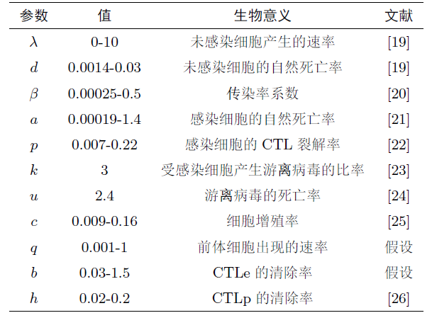
本节通过数值模拟验证理论分析结果, 我们选取初始值为(150,10,10,50,2)[18]. 首先, 针对无胞内时滞的情形, 基于表1 中的参数值, 计算系统在临界点处的规范型, 由此确定Hopf分支方向及分支周期解的稳定性. 同时, 借助规范性系数估计分支周期解的振幅与周期. 进一步, 通过对$(h,\tau)$ 双参数平面分支分析, 证明系统(1.2) 存在双Hopf 分支现象. 这一发现揭示了系统在特定参数组合下可能出现的复杂动力学行为.

表1   相关参数范围 (值) 表

新窗口打开| 下载CSV


5.1 Hopf分支

$\tau=0$ 时, 选取$h$ 作为分支参数, 研究免疫激活平衡点$E^{*}$ 处Hopf 分支的存在性. 固定参数$\lambda=1$, $d=0.03$, $\beta=0.005$, $a=0.001$, $p=0.001$, $c=0.01$, $q=0.05$, $b=0.08$, 令参数$h$ 变化. 根据定理4.6 的理论分析, 系统在此参数条件下可能出现Hopf 分支现象. 在该组参数下, 可得$\Delta_{4}(h)=0$ 存在唯一正实根$h_{1}\approx0.0594$, 该点是系统的Hopf分支临界点. 当$h\in(0.05,h_{1})$ 时, $\Delta_{4}(h)<0$, 平衡点$E^{*}$ 不稳定; 当$h\in(h_{1},0.15)$ 时, $\Delta_{4}(h)>0$, 平衡点$E^{*}$ 是局部渐近稳定的.

图1

图1   $\tau=0$ 时, 在平衡点$E^{*}$ 处以$h$ 为分支参数的分支图.


$h=h_{1}$ 时, 方程(4.9) 的特征根存在一对共轭纯虚根$\lambda_{1,2}=\pm0.0171743513 \mathrm{i}$ 以及三个负实根$\lambda_{3}=-0.0606009545$, $\lambda_{4}=-0.0302577275$$\lambda_{5}=-2.403633512$. 根据Hopf 分支理论, 这一特征根分布表明系统在$h=h_{1}$ 处发生Hopf 分支. 基于中心流行定理和规范性理论, 可进一步确定分支周期解的分支方向、周期解的稳定性、振幅和周期.

首先对系统(1.2) 进行坐标变换, 将平衡点$E^{*}$ 平移至坐标原点, 设参数$h=h_{1}+\epsilon$, 其中$\epsilon$ 为小扰动参数. 在此基础上, 通过线性变换将系统(1.2) 在平衡点处的雅可比矩阵为标准形式.

$\begin{equation}\label{5.1} \begin{aligned} \left( \begin{array}{c} x \\ y \\ v \\ w\\ z\\ \end{array} \right)=\left( \begin{array}{c} x^{*} \\ y^{*} \\ v^{*} \\ w^{*} \\ z^{*} \\ \end{array} \right)+P_{1}\left( \begin{array}{c} x_{1} \\ x_{2} \\ x_{3} \\ x_{4} \\ x_{5}\\ \end{array} \right), \end{aligned} \end{equation}$

这里

$\begin{equation*} \begin{aligned} \left( \begin{array}{c} x^{*} \\ y^{*} \\ v^{*} \\ w^{*}\\ z^{*}\\ \end{array} \right)=\left( \begin{array}{c} 32.06289867 \\ 8 \\ 10\\ 55.89733023\\ 3.764129982\\ \end{array} \right), \end{aligned} \end{equation*} $
$\begin{equation*} \begin{aligned} P_{1}\!=\!\!\!\left( \begin {array}{ccccc} 0.02205644693& 0.0046820354& 0.01515203330& 0.9976180153&- 0.001223792597\\ - 0.1608966834&- 0.1445430625& 0.1233057892&- 0.006747165032& 0.001210872103\\- 0.2024014936&- 0.1792287487& 0.1581249538&- 0.00854164429&- 0.9997529329\\- 4.711363429& 5.230465440&- 1.137352461& 0.1246453361&- 0.0002815924443\\ - 0.2867535380& 0.3669787859& 0.9185839340& 0.01063771240&- 0.00001395589018 \end{array} \right), \end{aligned} \end{equation*}$

系统(1.2) 被转换为

$\begin{equation*} \begin{aligned} \frac{\mathrm{d}x_{i}}{\mathrm{d}t}=F_{i}(x_{1},x_{2},x_{3},x_{4},x_{5};\epsilon),\quad i=1,2,3,4,5, \end{aligned} \end{equation*}$

其中

$\begin{align*} F_{1}&=0.0171743515x_{2}+[\epsilon(494174291700- 39765251950 x_{{1}}+ 46128202280 x_{{2}}\\ &~~~+ 122632148400x_{{3}}+ 13016697850 x_{{4}}- 11761767440 x_{{5}}+ 1127093083 x_{{2}}x_{{4}}\\ &~~~- 1146511453x_{{2 }}x_{{5}}+ 2841484016x_{{3}}x_{{4}}- 2869857319 x_{{3}}x_{{5}}- 33277537.88 x_{{4}}x_{{5}}\\ &~~~- 50347213.7 x_{{1}}x_{{2}}- 672141816.8x_{{1}} x_{{3}}- 891215429.8x_{{1}}x_{{4}}+ 895886332.5 x_{{1}}x_{{5}}\\ &~~~- 301962543.3 x_{{2}}x_{{3}}+ 161409593 {x_{{1}}}^{2}- 199925860.4{x_{{2}}}^{2}+ 496793691.1 {x_{{3}}}^{2}\\ &~~~+ 32839339.23{x_{{4}}}^{2}+ 43601.1{x_{{5}}}^{2})+O(\epsilon)+109596.4\,x_{{1}}{x_{{4}}}^{2}- 10264723.08\,{x_{{4}}}^{2}\\ &~~~- 97855812.1{x_{{5}}}^{2}- 1084766\, {x_{{1}}}^{3}+ 1005574.957\,{x_{{2}}}^{3}- 222505175.8\,{x_{{3}}}^{2}\\ &~~~+ 248755820.9\,{x_{{1}}}^{2}- 907106.3828\,{x_{{3}}}^{3}- 245525957.1\, {x_{{2}}}^{2}- 945823.9966\,x_{{1}}x_{{2}}x_{{4}}\\ &~~~- 2555645.183\,x_{{1} }x_{{2}}x_{{3}}+ 2144683.403\,x_{{1}}x_{{3}}x_{{4}}- 11044605.06\,x_{{ 2}}x_{{3}}x_{{5}}+ 445222.2408\,x_{{2}}x_{{4}}x_{{5}}\\ &~~~+ 1009343.602\,x_ {{1}}x_{{2}}x_{{5}}- 447005.5708\,x_{{3}}x_{{4}}x_{{5}}- 2221919.417\, x_{{1}}x_{{3}}x_{{5}}- 154420.4848\,x_{{1}}x_{{4}}x_{{5}}\\ &~~~+ 10792689.04 \,x_{{2}}x_{{3}}x_{{4}}- 5109261.09\,x_{{4}}{x_{{3}}}^{2}+ 5231163.09\,x_{{5}}{x_{{3}}}^{2}+ 390317.6486\,x_{{3}}{x_{{4}}}^{2}\\ &~~~+ 1329006.976\,x_{{1}}{x_{{3}}}^{2}- 42645039.9\,x_{{1}}x_{{5}}+ 1215147.294\,x_{{1}}{x_{{2}}}^{2}- 5628846.048\,{x_{{2}}}^{2}x_{{4}}\\ &~~~+ 27866339.97\,x_{{3}}x_{{5}}- 867869.4227\,{x_{{1}}}^{2}x_{{2}}- 28016321.9\,x_{{2}}x_{{4}}+ 410760927.9 \,x_{{2}}x_{{3}}\\ &~~~- 8720178.555\,x_{{1}}x_{{4}}- 6012726.997\,{x_{{1}}}^ {2}x_{{5}}+ 2828681.732\,x_{{2}}{x_{{3}}} ^{2}+ 641652.5417\,{x_{{1}}}^{2}x_{{3}}\\ &~~~+ 5929455.797\,{x_{{1}}}^{2}x_{ {4}}- 391575.6568\,x_{{2}}{x_{{4}}}^{2}- 2927220.373\,{x_{{2}}}^{2}x_{ {3}}- 33340872.6\,x_{{2}}x_{{5}}\\ &~~~- 49823950.33\,x_{{1}}x_{{2}}+5758208.919\,{x_{{2}}}^{2}x_{{5}}+ 99685628.45\,x_{{1}}x_{{3}}+ 26252933.5\,x_{{3}}x_{{4}}\\ &~~~- 62559715.4\,x_{{4}}x_{{5}}]/(- 420628986700+ 1803450467\,x_{{1}}+ 1745467133\,x_{{2}}\\&~~~- 1732769871\,x_{{3}}- 9890763710\,x_{{4}}+ 10009767250\,x_{{5}}),\\ F_{2}&=-0.01717435132\,x_{{1}}+[\epsilon( 786188393400- 63263063380\,x_{{1}}+ 73385964880\,x_{{2} }\\ &~~~\;+ 195097101000\,x_{{3}}+ 20708436150\,x_{{4}}- 18711950820\,x_{{5}}- 1824000180\,x_{{2}}x_{{5}}\\ &~~~\;- 480396189.6\,x_{{2}}x _{{3}}+ 1425277373\,x_{{1}}x_{{5}}- 1417846372\,x_{{1}}x_{{4}}- 1069319274\,x_{{1}}x_{{3}}\\ &~~~\;- 80098045.8\,x_{{1}}x_{{2}}- 52941673.54\,x_{{4}}x_{{5}}+ 4520554367\,x_{{3}}x_{{4}}- 4565693831\,x_{{3}}x_{{5}}\\&~~~\;+ 1793107239\,x_{{2}}x_{{4}}+ 790355630.4\,{x_{{3}}}^{2}- 318064686.1\,{x_{{2}}}^{2}+ 256788648.6\, {x_{{1}}}^{2}\\ &~~~\;+ 52244537.59\,{x_{{4}}}^{2} )+O(\epsilon)- 121887.465\,x_{{1}}{x_{{4}}}^{2}- 8421350.903\,{x_{{4}}}^{2}- 86564937.37\,{x_{{5}}}^{2}\\ &~~~\;+ 1586433.21\, {x_{{1}}}^{3}- 1568376.896\,{x_{{2}}}^{3}- 88220746.43\,{x_{{3}}}^{2}- 373809003.1\,{x_{{1}}}^{2}\\ &~~~\;- 355021.1147\,{x_{{3}}}^{3}+ 375163038.7\, {x_{{2}}}^{2}+ 1981978.621\,x_{{1}}x_{{2}}x_{{4}}- 330312.3617\,x_{{1} }x_{{2}}x_{{3}}\\ &~~~\;+ 9305063.264\,x_{{1}}x_{{3}}x_{{4}}+ 5258942.242\,x_{{ 2}}x_{{3}}x_{{5}}- 717019.7557\,x_{{2}}x_{{4}}x_{{5}}\\ &~~~\;- 2099340.559\,x_ {{1}}x_{{2}}x_{{5}}- 9409194.676\,x_{{1}}x_{{3}}x_{{5}}+ 186772.9312\, x_{{1}}x_{{4}}x_{{5}}- 5081227.149\,x_{{2}}x_{{3}}x_{{4}}\\ &~~~\;- 2039929.729 \,x_{{4}}{x_{{3}}}^{2}+ 2047447.381\,x_{{5}}{x_{{3}}}^{2}+ 2000894.995 \,x_{{1}}{x_{{3}}}^{2}- 33492421.7\,x_{{1}}x_{{5}}\\ &~~~\;- 1986935.005\,x_{{ 1}}{x_{{2}}}^{2}+ 8775247.215\,{x_{{2}}}^{2}x_{{4}}+ 25744891.38\,x_{{ 3}}x_{{5}}+ 1156796.172\,{x_{{1}}}^{2}x_{{2}}\\ &~~~\;+ 5236905.347\,x_{{3}}x_{ {4}}+ 16758640.71\,x_{{2}}x_{{4}}- 216631836.9\,x_{{2}}x_{{3}}- 16701633.1\,x_{{1}}x_{{4}}\\ &~~~\;+ 8793400.101\,{x_{{1}}}^{2}x_{{5}}- 55461334.2\,x_{{4}}x_{{5}}- 554417.3754\,x_{{2}}{x_{{3}}}^{2}- 3222195.662\,{x_{{1}}}^{2}x_{{3}}\\ &~~~\;- 8678680.676\,{x_{{1}}}^{2}x_{{4}}+ 632994.6131\,x_{{2}}{x_{{4}}}^{2}+ 2475691.029\,{x_{{2}}}^{2}x_{{3}}- 34260352.63\,x_{{2}}x_{{5}}\\ &~~~\;+ 81796167.1\,x_{{1}}x_{{2}}- 8980985.433 \,{x_{{2}}}^{2}x_{{5}}+ 401584732.3\,x_{{1}}x_{{3}}]/(- 420628986700\\ &~~~\;+ 1803450467\,x_{{1}}+ 1745467133\,x_{{2}}- 1732769871\,x_{{3}}- 9890763710\,x_{{4}}+ 10009767250\,x_{{5}}),\\ F_{3}&=- 0.06060095458\,x_{{3}}+[\epsilon(1564257883000- 125872814200\,x_{{1}}+ 146014079000\,x_{{2}}\\ &~~~\;+ 388179450200\,x_{{3}}+41203017960\,x_{{4}}- 37230664840 \,x_{{5}}+138014.9286\,{x_{{5}}}^{2}\\ &~~~\;- 3629164060\,x_{{2}}x _{{5}}- 955831366.9\,x_{{2}}x_{{3}}+ 2835836023\,x_{{1}}x_{{5}}- 2821050760\,x_{{1}}x_{{4}}\\ &~~~\;- 2127595775\,x_{{1}}x_{{3}}- 159368925.6\,x_{{1}}x_{{2}}- 105336622.8\,x_{{4}}x_{{5}}+ 8994425341\,x_{{3}}x_{{4}}\\ &~~~\;- 9084238117\,x_{{3}}x_{{5}}+ 3567697205\,x_{{2}}x_{{4}}+ 1572549323\,{x_{{3}}}^{2}- 632844744.1\,{x_{{2}}}^{2}\\ &~~~\;+ 510925461.8\,{x_{{1}}}^{2}+ 103949550\,{x_{{4} }}^{2} )+O(\epsilon)+18937.73732\,x_{{1}}{x_{{4}}}^{2}+ 384044.9765\,{x_{{4}}}^{2}\\ &~~~\;+ 4343491.371\,{x_{{5}}}^{2}- 228519.6664\, {x_{{1}}}^{3}+ 222404.1635\,{x_{{2}}}^{3}- 2159616.2\,{x_{{3}}}^{2}\\ &~~~\;+ 53489417.02\,{x_{{1}}}^{2}- 53453772.14\,{x_{{2}}}^{2}- 263970.6609\, x_{{1}}x_{{2}}x_{{4}}- 893063.2084\,x_{{1}}x_{{3}}x_{{4}}\\ &~~~\;- 1149166.915 \,x_{{2}}x_{{3}}x_{{5}}+ 100914.844\,x_{{2}}x_{{4}}x_{{5}}+ 279996.5834\,x_{{1}}x_{{2}}x_{{5}}+ 900258.3255\,x_{{1}}x_{{3}}x_{{5} }\\ &~~~\;+ 1116711.628\,x_{{2}}x_{{3}}x_{{4}}- 146409.2027\,x_{{1}}{x_{{3}}}^{ 2}+ 1421209.03\,x_{{1}}x_{{5}}+ 278666.9174\,x_{{1}}{x_{{2}}}^{2}\\ &~~~\;- 1244510.139\,{x_{{2}}}^{2}x_{{4}}- 170674.2445\,{x_{{1}}}^{2}x_{{2}}- 3293671.350\,x_{{2}}x_{{4}}+ 48131546.74\,x_{{2}}x_{{3}}\\ &~~~\;+ 1376286.028 \,x_{{1}}x_{{4}}- 1266656.084\,{x_{{1}}}^{2}x_{{5}}+ 2789841.213\,x_{{ 4}}x_{{5}}+ 208656.1073\,x_{{2}}{x_{{3}}}^{2}\\ &~~~\;+ 382038.6021\,{x_{{1}}}^ {2}x_{{3}}+ 1249877.303\,{x_{{1}}}^{2}x_{{4}}- 421516.2668\,{x_{{2}}}^ {2}x_{{3}}+ 2022457.624\,x_{{2}}x_{{5}}\\ &~~~\;- 11449072.88\,x_{{1}}x_{{2}}+ 1273550.966\,{x_{{2}}}^{2}x_{{5}}- 38174212.7\,x_{{1}}x_{{3}}/(- 420628986700\\ &~~~\;+ 1803450467x_{{1}}+ 1745467133x_{{2}}- 1732769871x_{{3}}- 9890763710x_{{4}}+ 10009767250x_{{5}}),\\ F_{4}&=- 0.03025772515\,x_{{4}}+[\epsilon(-38365505880+ 3087198248x_{{1}}- 3581189562\,x_{{2}}\\ &~~~+ 9520617503x_{{3}}- 1010558838x_{{4}}+ 913131591.9\,x_{{5}}+ 89010077.29\,x_{{2}}x_{{ 5}}+3384.999757\,{x_{{5}}}^{2}\\ &~~~+ 23443036.04\,x_{{2}}x_{{3}}- 69552651.62\,x_{{1}}x_{{5}}+ 69190023.41\,x_{{1}}x_{{4}}+ 52182117.22\,x_{{1}}x_{{3}}\\ &~~~+ 3908734.945 \,x_{{1}}x_{{2}}+ 2583520.828\,x_{{4}}x_{{5}}- 220600248.9\,x_{{3}}x_{ {4}}+ 222803026.7\,x_{{3}}x_{{5}}\\ &~~~- 87502520.89\,x_{{2}}x_{{4}}- 38568864.46\,{x_{{3}}}^{2}+ 15521359.37\,{x_{{2}}}^{2}- 12531126.75\, {x_{{1}}}^{2}\\ &~~~-2549501.024\,{x_{{4}}}^{2} )+O(\epsilon)- 16978204.20\,{x_{{5}}}^{2}+ 296560967.6\,{x_{{4}}}^{2}+ 4755158.493\,{x_{{3}}}^{2}\\ &~~~+ 3496995.496\, {x_{{2}}}^{2}- 5801498.241\,{x_{{1}}}^{2}+ 124972.9047\,x_{{4}}{x_{{3} }}^{2}- 103708.9453\,{x_{{2}}}^{2}x_{{5}}\\ &~~~+ 101392.1195\,{x_{{2}}}^{2}x _{{4}}+ 110217.5033\,{x_{{1}}}^{2}x_{{5}}- 108667.8343\,{x_{{1}}}^{2}x _{{4}}+ 8199552.781\,x_{{3}}x_{{5}}\\ &~~~- 2711042.3\,x_{{4}}x_{{5}}- 2771986.58\,x_{{2}}x_{{4}}- 1317600.091\,x_{{1}}x_{{2}}- 11079547.4 \,x_{{1}}x_{{5}}\\ &~~~- 1760431.612\,x_{{1}}x_{{3}}- 8557361.284\,x_{{2}}x_{ {3}}- 9632585.901\,x_{{2}}x_{{5}}- 3645302.92\,x_{{1}}x_{{4}}\\ &~~~+ 2231497.76\,x_{{3}}x_{{4}}- 127819.14\,x_{{5}}{x_{{3}}}^{2}- 233074.12\,x_{{2}}x_{{3}}x_{{4}}+ 238319.7\,x_{{2}}x_{{3}}x_{{5} }]\\&~~~/(-420628986700+ 1803450467x_{{1}}+ 1745467133x_{{2}}- 1732769871x_{{3}}\\&~~~- 9890763710x_{{4}}+ 10009767250x_{{5}}),\\ F_{5}&=- 2.403633513\,x_{{5}}+[\epsilon(6748400579- 543030776.4\,x_{{1}}+ 629922665.4\,x_{{2}}+ 1674653812\,x_{{3}}\\ &~~~+ 177754878.7\,x_{{4}}- 160617659.6\,x_{{5}}+595.4133484{x_{{5}}}^{2}- 15656659.37x_{{2}}x_{{5 }}\\ &~~~- 4123573.883x_{{2}}x_{{3}}+ 12234144.81x_{{1}}x_{{5}}- 12170359.37x_{{1}}x_{{4}}- 9178709.419x_{{1}}x_{{3}}\\ &~~~- 687537.1135 x_{{1}}x_{{2}}- 454435.1247x_{{4}}x_{{5}}+ 38803055.32x_{{3}}x_{ {4}}- 39190518.65x_{{3}}x_{{5}}\\ &~~~+ 15391483.81x_{{2}}x_{{4}}+ 6784170.867{x_{{3}}}^{2}- 2730169.932{x_{{2}}}^{2}+ 2204195.178\, {x_{{1}}}^{2}\\ &~~~+ 448451.1228\,{x_{{4}}}^{2} )+O(\epsilon)+3671739.183\,{x_{{4}}}^{2}+ 36243520 \,{x_{{5}}}^{2}- 101105.6603\,{x_{{1}}}^{3}\\ &~~~+ 112918.6\,{x_{{2}}}^{3 }+ 60479913.29\,{x_{{3}}}^{2}+ 25170856.46\,{x_{{1}}}^{2}- 26026742.33 \,{x_{{2}}}^{2}\\ &~~~- 205713.7862\,x_{{1}}x_{{2}}x_{{4}}+ 560490.2644\,x_{{ 1}}x_{{2}}x_{{3}}- 2242906.015\,x_{{1}}x_{{3}}x_{{4}}\\ &~~~+ 1109417.415\,x_ {{2}}x_{{3}}x_{{5}}+ 216437.9619\,x_{{1}}x_{{2}}x_{{5}}+ 2278330.324\, x_{{1}}x_{{3}}x_{{5}}\\&~~~- 1095454.238\,x_{{2}}x_{{3}}x_{{4}}+ 1391401.9 \,x_{{4}}{x_{{3}}}^{2}- 1416519.334\,x_{{5}}{x_{{3}}}^{2}- 650603.5793 \,x_{{1}}{x_{{3}}}^{2}\\&~~~+ 15003372\,x_{{1}}x_{{5}}+ 154454.962\,x_{{1 }}{x_{{2}}}^{2}- 631299.868\,{x_{{2}}}^{2}x_{{4}}- 10541813\,x_{{3} }x_{{5}}\\ &~~~- 6146085.983\,x_{{3}}x_{{4}}+ 2129989.376\,x_{{2}}x_{{4}}- 48693788.89\,x_{{2}}x_{{3}}+ 4962849.16\,x_{{1}}x_{{4}}\\ &~~~- 560415.0051 \,{x_{{1}}}^{2}x_{{5}}+ 23194340\,x_{{4}}x_{{5}}- 439733.1382\,x_{{2 }}{x_{{3}}}^{2}+ 508210.3039\,{x_{{1}}}^{2}x_{{3}}\\ &~~~+ 554040.2462\,{x_{{ 1}}}^{2}x_{{4}}+ 13334859.0\,x_{{2}}x_{{5}}- 6361098.163\,x_{{1}}x_{{2 }}+ 646606.4835\,{x_{{2}}}^{2}x_{{5}}\\ &~~~- 98205550.19\,x_{{1}}x_{{3}}]/(- 420628986700+ 1803450467x_{{1}}+ 1745467133x_{{2}}\\ &~~~- 1732769871x_{{3}}- 9890763710x_{{4}}+ 10009767250x_{{5}}). \end{align*}$

可得系统(1.2) 在平凡平衡点$x_{i}=0(i=1,2,3)$ 处的雅可比矩阵为

$\begin{equation*} \begin{aligned} J=\left( \begin{array}{ccccc} 0 & 0.0171743513 & 0&0&0 \\ -0.0171743513 & 0 & 0 &0&0\\ 0 & 0 &-0.0606009545&0&0 \\ 0 & 0 &0&-0.03025772515&0 \\ 0 & 0 &0&0& -2.403633513 \\ \end{array} \right). \end{aligned} \end{equation*}$

通过极坐标变换, 可将系统表示为规范型

$\begin{equation}\label{5.2} \begin{aligned} \frac{\mathrm{d}r}{\mathrm{d}\bar{t}}&=r(\nu_{0}\epsilon+\nu_{1}r^{2})+O(\epsilon^{2}r,\epsilon r^{3},r^{5}),\\ \frac{\mathrm{d}\theta}{\mathrm{d}\bar{t}}&=\omega_{0}+\vartheta_{0}\epsilon+\vartheta_{1}\epsilon^{2}+O(\epsilon^{2},\epsilon r^{2},r^{4}). \end{aligned} \end{equation}$

其中$\omega_{0}=0.01717435132$ 对应方程(4.9) 的一对纯虚特征值. 基于文献[27] 中的理论, 可计算得一阶系数

$\begin{equation*} \begin{aligned} &\nu_{0}=\frac{1}{2}\left(\frac{\partial^{2}F_{1}}{\partial x_{1}\partial\epsilon}+\frac{\partial^{2}F_{2}}{\partial x_{2}\partial\epsilon}\right)\bigg|_{\epsilon=0,x_{i}=0}=-0.0463614075,\\ &\vartheta_{0}=\frac{1}{2}\left(\frac{\partial^{2}F_{1}}{\partial x_{2}\partial\epsilon}-\frac{\partial^{2}F_{2}}{\partial x_{1}\partial\epsilon}\right)\bigg|_{\epsilon=0,x_{i}=0}=-0.1284637228. \end{aligned} \end{equation*}$

进一步应用文献[27] 中的Maple 程序计算高阶项系数

$\nu_{1}=-0.0000024658,\quad\quad\quad\vartheta_{1}=-0.000000035.$

因此, 系统(5.2)的三阶规范型为

$\begin{equation}\label{5.3} \begin{aligned} \frac{\mathrm{d}r}{\mathrm{d}\bar{t}}&=r(-0.0463614075\epsilon-0.0000024658r^{2}),\\ \frac{\mathrm{d}\theta}{\mathrm{d}\bar{t}}&= 0.0171743513-0.1284637228\epsilon-0.000000035r^{2}. \end{aligned} \end{equation}$

在系统(5.3)中, 令$\mathrm{d}r/\mathrm{d}\bar{t}=\mathrm{d}\theta/\mathrm{d}\bar{t}=0$ 可求得稳态解, 解得 $r=0$, $r^{2}=18801.77123$. 其中, 零解$r=0$ 对应于系统(1.2) 的平衡点$E^{*}$. 通过对$\mathrm{d}r/\mathrm{d}\bar{t}$ 进行线性稳定性分析表明, 当$\epsilon>0$ 时, 平衡点$\bar{r}=0$ 是稳定的. 当$\epsilon$ 从负值增加到零时, 出现Hopf 分支, 此时周期解的振幅由非零稳态解给出

$r=137.1417997\sqrt{-\epsilon},\quad\epsilon<0.$

由于$\nu_{1}<0$, 可知该Hopf 分支是超临界分支, 且分支产生的极限环是稳定的. 此外, 分支极限环的振幅为$r=137.1417997\sqrt{-\epsilon}$, 频率为

$\omega=0.0171743513-0.1284637228\epsilon.$

5.2 双Hopf分支

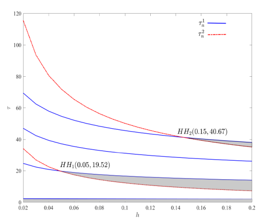
本小节研究时滞参数$\tau>0$ 时系统的动力学行为, 选取参数如下: $\lambda=10$, $d=0.0014$, $\beta=0.45$, $a=0.3$, $p=0.001$, $c=0.15$, $q=0.35$, $b=1.4$. 通过对双参数$(h,\tau)$的分支分析, 得到如图2 所示的Hopf 分支曲线, 可以发现当参数组合$(h,\tau)=HH_{i}(i=1,2)$ 时, 系统在平衡点$E^{*}$处出现双Hopf分支. 特别地, 当固定$h$ 并逐渐增大$\tau$ 时, $E^{*}$ 的稳定性将会出现开关现象. 以$h=0.17$ 为例, 随着$\tau$ 的增加, $E^{*}$ 的稳定性改变5次. 且前几个分支值依次为

$\begin{align*} \tau_{0}^{1}=1.9938<\tau_{0}^{2}=8.2287<\tau_{1}^{1}=14.5495<\tau_{2}^{1}=27.0992<\tau_{1}^{2}=38.1437<\tau_{3}^{1}=39.6489. \end{align*}$

进一步计算可得$\omega_{1}\approx0.5007 > \omega_{2}\approx0.21 $. 基于此, 当 $\tau\in[0,\tau_{0}^{1})\cup(\tau_{0}^{2},\tau_{1}^{1})\cup(\tau_{1}^{2},\tau_{3}^{1})$ 时, $E^{*}$ 是稳定的; 当$\tau\in(\tau_{0}^{1},\tau_{0}^{2})\cup(\tau_{1}^{1},\tau_{1}^{2})$ 时, $E^{*}$ 是不稳定的. 且在后一种情形下, 系统 (1.2) 至少有一个周期解.

图2

图2   $E^{*}$ 的稳定性区域分布示意图 (阴影部分为稳定区域, 白色为不稳定区域), 其中$HH_{1},HH_{2}$ 是双Hopf分支点.


6 结论

本研究基于具有病毒-细胞感染、胞内时滞和CTL 免疫反应机制的HIV 感染动力学模型, 开展了系统的理论分析和数值模拟研究. 通过构造合适的Lyapunov 泛函, 建立了系统平衡点的全局稳定性判据, 揭示了不同感染状态下的病毒动力学特征. 研究结果表明, 当免疫失活再生数$\mathcal{R}_0<1$ 时, 未感染平衡点全局渐近稳定, 病毒最终被完全消除; 当免疫失活再生数$\mathcal{R}_0>1$ 而免疫激活再生数$\mathcal{R}_1<1$ 时, 免疫失活平衡点呈现全局渐近稳定性, 此时系统将趋向病毒持续存在但免疫应答未被充分激活的状态.

进一步研究表明, 系统在特定参数范围内会出现Hopf 分支, 甚至可能产生更复杂的双Hopf 分支. 在无胞内时滞情形下, 通过规范性计算精确刻画了分支周期解的分支方向、稳定性等性质, 并得到了分支周期解的振幅和周期; 在考虑胞内时滞的情形下, 通过双参数分支分析验证了双Hopf分支的存在性. 这些研究结果为深入理解HIV 感染的免疫动力学机制提供了重要的理论依据.

参考文献

Duffin R P, Tullis R H.

Mathematical models of the complete course of HIV infection and AIDS

J Theor Med, 2002, 4(4): 215-221

[本文引用: 1]

Ho D, Neumann A, Perelson A, et al.

Rapid turnover of plasma virions and CD4 lymphocytes in HIV-1 infection

Nature, 1995, 373(6510): 123-126

DOI:10.1038/373123a0      [本文引用: 1]

Narayan O, Kennedy S, Shelfer D, et al.

Activation of caprine arthritis-encephalitis virus expression during maturation of monocytes to macrophages

Infect Immun, 1983, 41(1): 67-73

DOI:10.1128/iai.41.1.67-73.1983      PMID:6862634      [本文引用: 1]

Lentiviruses, which cause arthritis-encephalitis and maedi-visna in goats and sheep, respectively, cause persistent infections in these animals. The viruses replicate productively at low levels in macrophages in diseased organs such as the "maedi lung" and nonproductively in other cell types such as leukocytes in peripheral blood. Nonproductive infections become productive during in vitro cultivation of the cells. This study showed that monocytes were the only cells in the peripheral blood leukocytes of an infected animal in which virus was detected and that virus activation occurred only when these cells matured into macrophages. Only a minute fraction of cultured monocytes matured into macrophages, and viral infectivity was associated exclusively with this fraction. Antiglobulin-coated glass wool fragments were lethal for monocyte macrophages because of toxic phagocytosis, but had no effect on B or T lymphocytes. The simultaneous addition of the glass fragments and leukocytes to culture dishes resulted in no macrophage maturation and no virus production. The addition of the fragments to virus-producing macrophages caused the death of the cells and a decline in virus production. Virus production in less avidly phagocytic cells was unaffected by the glass. Thus, although macrophages may be permissive for virus replication, one mechanism for restricted virus expression in vivo may be physiological factors controlling the maturation of these cells.

Gluckman J C, Klatzmann D, Montagnier L.

Lymphadenopathy-associated-virus infection and acquired immunodeficiency syndrome

Ann Rev Immunol, 1986, 4: 97-117

DOI:10.1146/immunol.1986.4.issue-1      URL     [本文引用: 1]

Wodarz D. Killer Cell Dynamics:Mathematical and Computational Approaches to Immunology. New York: Springer-Verlag, 2007

[本文引用: 1]

Doherty P C, Topham D J, Tripp R A.

Establishment and persistence of virus-specific CD4$^{+}$ and CD8$^{+}$ T cell memory

Immunol Rev, 1996, 150(1): 23-44

DOI:10.1111/imr.1996.150.issue-1      URL     [本文引用: 1]

Ahmed R, Gray D.

Immunological memory and protective immunity: understanding their relation

Science, 1996, 272(5258): 54-60

DOI:10.1126/science.272.5258.54      PMID:8600537     

The immune system can remember, sometimes for a lifetime, the identity of a pathogen. Understanding how this is accomplished has fascinated immunologists and microbiologists for many years, but there is still considerable debate regarding the mechanisms by which long-term immunity is maintained. Some of the controversy stems from a failure to distinguish between effector and memory cells and to define their roles in conferring protection against disease. Here the current understanding of the cellular basis of immune memory is reviewed and the relative contributions made to protective immunity by memory and effector T and B cells are examined.

Zinkernagel R M, Bachmann M F, Kundig T M.

On immunological memory

Annu Rev Immunol, 1996, 14(1): 333-367

DOI:10.1146/immunol.1996.14.issue-1      URL     [本文引用: 1]

Lau L L, Jamieson B D, Somasundaram T.

Cytotoxic T-cell memory without antigen

Nature, 1994, 369(6482): 648-652

DOI:10.1038/369648a0      [本文引用: 1]

Kundig T M, Bachmann M F, Oehen S.

On the role of antigen in maintaining cytotoxic T-cell memory

Proc Natl Acad SCI USA, 1996, 93(18): 9716-9723

PMID:8790397      [本文引用: 1]

This study evaluated whether T-cell memory reflects increased precursor frequencies of specific long-lived T cells and/or a low-level immune response against some form of persistent antigen. Antivirally protective CD8+ T-cell memory was analyzed mostly in the original vaccinated host to assess the role of antigen in its maintenance. T-cell mediated resistance against reinfection was measured in the spleen and in peripheral solid organs with protocols that excluded protection by antibodies. In vivo protection was compared with detectable cytotoxic T-lymphocyte precursor frequencies determined in vitro. In the spleen, in vitro detectable cytotoxic T-lymphocyte precursor frequencies remained stable independently of antigen, conferring resistance against viral replication in the spleen during reinfection. In contrast, T-cell mediated resistance against reinfection of peripheral solid organs faded away in an antigen-dependent fashion within a few days or weeks. We show that only memory T cells persistently or freshly activated with antigen efficiently extravasate into peripheral organs, where cytotoxic T lymphocytes must be able to exert effector function immediately; both the capacity to extravasate and to rapidly exert effector function critically depend on restimulation by antigen. Our experiments document that the duration of T-cell memory protective against peripheral reinfection depended on the antigen dose used for immunization, was prolonged when additional antigen was provided, and was abrogated after removal of antigen. We conclude that T-cell mediated protective immunity against the usual peripheral routes of reinfection is antigen-dependent.

Jamieson B D, Ahmed R.

Long term persistence of virus-specific cytotoxic T cells

J Exp Med, 1989, 169(6): 1993-2005

DOI:10.1084/jem.169.6.1993      PMID:2471771      [本文引用: 1]

This study documents that virus-specific CTL can persist indefinitely in vivo. This was accomplished by transferring Thy-1.1 T cells into Thy-1.2 recipient mice to specifically identify the donor T cell population and to characterize its antigenic specificity and function by using a virus-specific CTL assay. Thy-1.1+ T cells from mice previously immunized with lymphocytic choriomeningitis virus (LCMV) were transferred into Thy-1.2 mice persistently infected with LCMV. The transferred LCMV-specific CTL (Thy-1.1+ CD8+) eliminate virus from the chronically infected carriers and persist in the recipient mice in small numbers, comprising only a minor fraction of the total T cells. Upon re-exposure to virus, these long-lived "resting" CD8+ T cells proliferate in vivo to become the predominant cell population. These donor CD8+ T cells can be recovered up to a year post-transfer and still retain antigenic specificity and biological function. They kill LCMV infected H-2-matched cells in vitro and can eliminate virus upon transfer into a second infected host. In addition, these long-lived CD8+ T cells appear not to be dependent on help from CD4+ T cells, since depletion of CD4+ T cells has minimal or no effect on their biological properties (proliferation, CTL response, viral clearance). These donor CTL also exhibit an immunodominance over the host-derived LCMV-specific CTL response. When both host and donor T cells are present, the donor CTL response is dominant over the potential CTL response of the cured carrier host. Taken together, these results suggest that virus-specific CTL can persist for the life span of the host as memory cells.

Oehen S, Brduscha-Riem K.

Differentiation of naive CTL to effector and memory CTL: correlation of effector function with phenotype and cell division

J Immunol, 1998, 161(10): 5338-5346

PMID:9820507      [本文引用: 1]

Phenotypically and functionally, the early steps of T cell differentiation are not well characterized. In addition, the effector T cell stage shares several phenotypic characteristics with memory T cells, which has made the analysis of T cell memory difficult. In this study, we have investigated in vitro and in vivo the differentiation of naive CTL into effector and memory CTL as a function of cell division using lymphocytic choriomeningitis virus-specific TCR-transgenic spleen cells labeled with the vital dye carboxyfluorescein diacetate, succinimidyl ester. The following major points emerged. 1) During the first nine cell divisions, the investigated cell surface markers were strongly modulated. 2) The TCR was stepwise down-regulated during viral infection. 3) Cytotoxic effector function was acquired within one cell division and was retained during the next four to five divisions. 4) In vitro, CTL reached a CD44highCD62L+ memory phenotype after 6-10 cell divisions and required restimulation to exert effector function. 5) Lymphocytic choriomeningitis virus memory mice contained two distinct memory populations: a CD44highCD62L- population, predominately located in the spleen and exerting rapid effector function, and a CD44highCD62L+ population found in the spleen and the lymph nodes, which had lost immediate effector function. This finding suggests that two types of memory CTL exist. The correlation between CD62L expression, effector function, and Ag persistence is discussed.

Wodarz D, May R M, Nowak M A.

The role of antigen-independent persistence of memory cytotoxic T lymphcytes

Inter Immunol, 2000, 12(4): 467-477

DOI:10.1093/intimm/12.4.467      URL     [本文引用: 2]

Li M Y, Wang L C.

Backward bifurcation in a mathematical model for HIV infection in vivo with anti-retroviral treatment

Nonlin Anal Real World Appl, 2014, 17: 147-160

DOI:10.1016/j.nonrwa.2013.11.002      URL     [本文引用: 2]

Yu P.

Closed-form conditions of bifurcation points for general differential equations

Int J Bifurcation and Chaos, 2005, 15(04): 1467-1483

DOI:10.1142/S0218127405012582      URL     [本文引用: 1]

This note presents closed-form formulas for determining the critical points of general n-dimensional differential equations. The formulas do not require commutating the eigenvalues of the Jacobian of a system. Based on the Hurwitz criterion, explicit necessary and sufficient conditions are obtained. Particular attention is focused on Hopf and double Hopf bifurcations. A model of induction machine is presented to show the application of the results.

Beretta E, Kuang Y.

Geometric stability switch criteria in delay differential systems with delay dependent parameters

SIAM J Appl Math, 2002, 33(5): 1144-1165

Nelson P W, Murray J D, Perelson A S.

A model of HIV-1 pathogenesis that includes an intracellular delay

Math Biosci, 2002, 163(2): 201-215

DOI:10.1016/S0025-5564(99)00055-3      URL     [本文引用: 1]

Prakash M, Balasubramaniam P.

Bifurcation analysis of macrophages infection model with delayed immune response

Commun Nonlinear Sci, 2016, 35: 1-16

DOI:10.1016/j.cnsns.2015.10.012      URL     [本文引用: 1]

Adak D, Bairagi N.

Analysis and computation of multi-pathways and multi-delays HIV-1 infection model

Appl Math Model, 2018, 54: 517-536

DOI:10.1016/j.apm.2017.09.051      URL    

Li B, Chen Y, Lu X, et al.

A delayed HIV-1 model with virus waning term

Math Biosci Eng, 2016, 13(1): 135-157

DOI:10.3934/mbe.2016.13.135      PMID:26776264     

In this paper, we propose and analyze a delayed HIV-1 model with CTL immune response and virus waning. The two discrete delays stand for the time for infected cells to produce viruses after viral entry and for the time for CD8+ T cell immune response to emerge to control viral replication. We obtain the positiveness and boundedness of solutions and find the basic reproduction number R0. If R0 < 1, then the infection-free steady state is globally asymptotically stable and the infection is cleared from the T-cell population; whereas if R0 > 1, then the system is uniformly persistent and the viral concentration maintains at some constant level. The global dynamics when R0 > 1 is complicated. We establish the local stability of the infected steady state and show that Hopf bifurcation can occur. Both analytical and numerical results indicate that if, in the initial infection stage, the effect of delays on HIV-1 infection is ignored, then the risk of HIV-1 infection (if persists) will be underestimated. Moreover, the viral load differs from that without virus waning. These results highlight the important role of delays and virus waning on HIV-1 infection.

Asquith B, Mosley A J, Barfield A, et al.

A functional CD$8^{+}$ cell assay reveals individual variation in CD$8^{+}$ antiviral efficacy and explains differences in human T-lymphotropic virus type 1 proviral load

J Gen Virol, 2005, 86: 1515-1523

DOI:10.1099/vir.0.80766-0      PMID:15831965     

The CD8+ lymphocyte response is a main component of host immunity, yet it is difficult to quantify its contribution to the control of persistent viruses. Consequently, it remains controversial as to whether CD8+ cells have a biologically significant impact on viral burden and disease progression in infections such as human immunodeficiency virus-1 and human T-lymphotropic virus type I (HTLV-I). Experiments to ascertain the impact of CD8+ cells on viral burden based on CD8+ cell frequency or specificity alone give inconsistent results. Here, an alternative approach was developed that directly quantifies the impact of CD8+ lymphocytes on HTLV-I proviral burden by measuring the rate at which HTLV-I-infected CD4+ cells were cleared by autologous CD8+ cells ex vivo. It was demonstrated that CD8+ cells reduced the lifespan of infected CD4+ cells to 1 day, considerably shorter than the 30 day lifespan of uninfected cells in vivo. Furthermore, it was shown that HTLV-I-infected individuals vary considerably in the rate at which their CD8+ cells clear infected cells, and that this was a significant predictor of their HTLV-I proviral load. Forty to 50 % of between-individual variation in HTLV-I proviral load was explained by variation in the rate at which CD8+ cells cleared infected cells. This novel approach demonstrates that CD8+ cells are a major determinant of HTLV-I proviral load. This assay is applicable to quantifying the CD8+ cell response to other viruses and malignancies and may be of particular importance in assessing vaccines.

Yang Y, Zou L, Ruan S.

Global dynamics of a delayed within-host viral infection model with both virus-to-cell and cell-to-cell transmissions

Math Biosci, 2015, 270: 183-191

DOI:10.1016/j.mbs.2015.05.001      PMID:25998145     

A within-host viral infection model with both virus-to-cell and cell-to-cell transmissions and three distributed delays is investigated, in which the first distributed delay describes the intracellular latency for the virus-to-cell infection, the second delay represents the intracellular latency for the cell-to-cell infection, and the third delay describes the time period that viruses penetrated into cells and infected cells release new virions. The global stability analysis of the model is carried out in terms of the basic reproduction number R0. If R0≤1, the infection-free (semi-trivial) equilibrium is the unique equilibrium and is globally stable; if R0>1, the chronic infection (positive) equilibrium exists and is globally stable under certain assumptions. Examples and numerical simulations for several special cases are presented, including various within-host dynamics models with discrete or distributed delays that have been well-studied in the literature. It is found that the global stability of the chronic infection equilibrium might change in some special cases when the assumptions do not hold. The results show that the model can be applied to describe the within-host dynamics of HBV, HIV, or HTLV-1 infection. Copyright © 2015. Published by Elsevier Inc.

Culshaw R V, Ruan S.

A delay-differential equation model of HIV infection of CD$4^{+}$ T cells

Math Biosci, 2000, 165(1): 27-39

PMID:10804258     

A.S. Perelson, D.E. Kirschner and R. De Boer (Math. Biosci. 114 (1993) 81) proposed an ODE model of cell-free viral spread of human immunodeficiency virus (HIV) in a well-mixed compartment such as the bloodstream. Their model consists of four components: uninfected healthy CD4(+) T-cells, latently infected CD4(+) T-cells, actively infected CD4(+) T-cells, and free virus. This model has been important in the field of mathematical modeling of HIV infection and many other models have been proposed which take the model of Perelson, Kirschner and De Boer as their inspiration, so to speak (see a recent survey paper by A.S. Perelson and P.W. Nelson (SIAM Rev. 41 (1999) 3-44)). We first simplify their model into one consisting of only three components: the healthy CD4(+) T-cells, infected CD4(+) T-cells, and free virus and discuss the existence and stability of the infected steady state. Then, we introduce a discrete time delay to the model to describe the time between infection of a CD4(+) T-cell and the emission of viral particles on a cellular level (see A.V.M. Herz, S. Bonhoeffer, R.M. Anderson, R.M. May, M.A. Nowak [Proc. Nat. Acad. Sci. USA 93 (1996) 7247]). We study the effect of the time delay on the stability of the endemically infected equilibrium, criteria are given to ensure that the infected equilibrium is asymptotically stable for all delay. Numerical simulations are presented to illustrate the results.

Asquith B, Bangham C R M.

Quantifying HTLV-I dynamics

Immunol Cell Biol, 2007, 85(4): 280-286

PMID:17372609     

Despite significant advances in our understanding of the immune response to persistent viruses like human T-cell lymphotropic virus type I (HTLV-I), many important questions remain unanswered. Mathematical modelling enables us to interpret and synthesise diverse experimental data in new ways and thus can contribute to our understanding. Here, we review recent advances in mathematical modelling of HTLV-I infection and illustrate how mathematics has enabled us to identify factors that determine an individual's viral burden and risk of developing HTLV-I-associated diseases.

Perelson A S, Kirschner D E, De Boer S R.

Dynamics of HIV infection of CD4$^{+}$ T cells

Math Biosci, 1993, 114(1): 81-125

PMID:8096155     

We examine a model for the interaction of HIV with CD4+ T cells that considers four populations: uninfected T cells, latently infected T cells, actively infected T cells, and free virus. Using this model we show that many of the puzzling quantitative features of HIV infection can be explained simply. We also consider effects of AZT on viral growth and T-cell population dynamics. The model exhibits two steady states, an uninfected state in which no virus is present and an endemically infected state, in which virus and infected T cells are present. We show that if N, the number of infectious virions produced per actively infected T cell, is less a critical value, Ncrit, then the uninfected state is the only steady state in the nonnegative orthant, and this state is stable. For N > Ncrit, the uninfected state is unstable, and the endemically infected state can be either stable, or unstable and surrounded by a stable limit cycle. Using numerical bifurcation techniques we map out the parameter regimes of these various behaviors. oscillatory behavior seems to lie outside the region of biologically realistic parameter values. When the endemically infected state is stable, it is characterized by a reduced number of T cells compared with the uninfected state. Thus T-cell depletion occurs through the establishment of a new steady state. The dynamics of the establishment of this new steady state are examined both numerically and via the quasi-steady-state approximation. We develop approximations for the dynamics at early times in which the free virus rapidly binds to T cells, during an intermediate time scale in which the virus grows exponentially, and a third time scale on which viral growth slows and the endemically infected steady state is approached. Using the quasi-steady-state approximation the model can be simplified to two ordinary differential equations the summarize much of the dynamical behavior. We compute the level of T cells in the endemically infected state and show how that level varies with the parameters in the model. The model predicts that different viral strains, characterized by generating differing numbers of infective virions within infected T cells, can cause different amounts of T-cell depletion and generate depletion at different rates. Two versions of the model are studied. In one the source of T cells from precursors is constant, whereas in the other the source of T cells decreases with viral load, mimicking the infection and killing of T-cell precursors.(ABSTRACT TRUNCATED AT 400 WORDS)

Yu P, Huseyin K.

A perturbation analysis of interactive static and dynamical bifurcation

IEEE Trans Automat Contr, 2002, 33(1): 28-41

DOI:10.1109/9.358      URL    

Yu P.

Computation of normal forms via a perturbation technique

J Sound Vibr, 1998, 211(1): 19-38

DOI:10.1006/jsvi.1997.1347      URL     [本文引用: 2]

/