种群动力学主要研究的是生活在同一栖息地的特定生物群体、物种或物种系统数量随时间的变化规律. 物种数量的增减, 比如出生、繁殖和死亡的速度, 既受环境因素影响, 像种群自身密度、食物供应量, 以及基因决定的特性等, 也与同栖息地其他物种的特性密切相关. 在生态系统中, 弄清楚物种数量如何变化至关重要, 因为这有助于我们更有效地管理和控制物种, 以进一步维护生态平衡^[1-3].

在生态系统里, 种群间的相互作用主要有三种: 共生, 捕食与被捕食以及竞争^[4-6]. 其中, 捕食者与被捕食者之间的关系尤为复杂且引人关注^[7-9]. 这种关系的动力学特征, 包括稳定性、周期性变化、分岔现象, 甚至混沌行为, 它们都是生态学研究的热点. 事实上, 自然界中大多数生物都处在食物链中, 要么是捕食者, 要么是被捕食者. 如果我们能深入理解这两者之间的数量关系, 就能更好地调控它们的数量, 防止某一物种数量过多或过少, 从而避免对整个生态系统造成破坏.

在生物学中, 捕食者与被捕食者之间的数量关系被称作捕食者-食饵模型. 近几十年来, 这类模型一直受到生物学家和数学家们的广泛关注^[10-12], 并不断努力构建更贴近现实的模型. 从应用数学的角度, 我们会运用动力学理论来分析这些模型, 讨论它们是否符合数学逻辑, 进而通过动力学的研究方法揭示出它们的生物学意义, 让这些模型在生态学研究和实践中发挥更大作用. 这样, 我们就能更准确地预测和调控生物种群的数量, 保护生态系统的稳定与和谐.

假设现在有两个物种$x_n, y_n$按照logistics型动力学演化. 如果它们共享同一个生态系统并相互作用, 我们可以通过如下耦合系统来近似它们的演化^[13-15]

两个物种之间的相互作用导致生长速率$\mu(z)$随时间变化. 因此, $\mu(z)$依赖于其他种群的种群规模. 这种增长率的最简单的选择可以是线性增加的函数$\mu_1$或线性减少的函数$\mu_2$, 因此, 设$ \mu_1(z)=\lambda_1(3 z+1)$, $\mu_2(z)=\lambda_2(-3 z+4)$, 并针对物种间的三种不同关系, 我们可以得到三种不同的模型

(i) 共生因互惠而产生对称耦合, 则$\mu_x=\mu_y=\mu_1$;

(ii) 捕食者-食饵相互作用是基于捕食者和食饵之间分别建立的利益/损害关系, 则$\mu_x=\mu_1$ 和$\mu_y=\mu_2$;

(iii) 物种间的竞争导致相反的对称耦合, 则$\mu_x=\mu_y=\mu_2$. 2009 年, López-Ruiz 和 Fournier-Prunaret^[15] 考虑了第三种物种关系, 即系统 (1.1) 满足如下对称耦合关系

其中, $\lambda$表示竞争强度, 耦合项$(-3z + 4)$反映物种间的相互抑制(竞争导致增长率下降). 他们用数值模拟的方法确定了竞争强度参数$\lambda \in(0.25,1.206)$内系统稳定性的定量映射关系(如当$\lambda=0.9811$时周期$2$轨道生成), 分析了系统(1.2)随$\lambda$变化时吸引子的类型演替(从固定点到周期轨道, 再到不变闭曲线, 最后到混沌)及对应的分岔点参数阈值, 还揭示了竞争作用通过诱导多稳态、高周期震荡与混沌动力学促进生物多样性的机制, 并展现了吸引域边界的分形结构对初始条件的敏感依赖性.

本文我们讨论第二种物种关系, 建立logistics型捕食者-食饵相互作用的动态交互, 即如下二维离散系统

其中$a, b$均大于$0$, $x_n$和$y_n$分别代表离散时间步长$n$下的食饵和捕食者的标准化种群密度, 时间间隔可以方便地取为一年. 在综合考虑物种出生率、繁殖率、死亡率、自身密度、食物资源、遗传特性以及共生物种相互作用等多重生态因素的基础上, 食饵的自然增长率并非简单的参数$a$, 而是依赖于捕食者数量$y_n$的复合项$a(3y_n + 1)$, 这意味着捕食者的存在显著影响食饵的增长潜力, 同理, 捕食者的自然增长率也是依赖于食饵数量$x_n$的复合项$b(- 3x_n + 4)$, 即食饵数量亦直接影响捕食者的增长潜力. 因此, 系统(1.3)的两个增长项一个依赖于捕食者且正向相关, 一个依赖于食饵但负向相关. 与大多数经典的捕食者-食饵模型显著不同, 在分析其动力学行为时, 需要特别注意这些非典型结构的影响. 值得注意的是, 该模型在$x_n, ~y_n \in [0,1]$的标准化密度范围内定义良好: $x_n=0$ 或$1$分别对应食饵灭绝或饱和状态, $y_n$同理, 这一设定既约束了种群密度的数学有界性, 亦映射了生态系统中环境承载力的物理限制.

本文主要在$x_n, ~y_n \in [0,1]$的范围内研究系统(1.3)的动力学行为, 包括在各个不动点附近的跨临界和翻转分岔, 以及Marotto 意义下混沌的存在性. 具体地, 在第二节中, 我们运用多项式完全判别系统理论^[16,17]给出系统(1.3)中的三个不动点的拓扑分类及其稳定性. 第三节中, 我们讨论系统(1.3)在平凡不动点$O$附近的分岔类型, 并证明随着参数的变化, 系统在$O$附近能够发生跨临界分岔. 在第四节我们考虑系统(1.3)在不动点$E_1$和$E_2$附近的分岔类型, 并给出系统在$E_1$和$E_2$附近发生跨临界和翻转分岔的参数条件. 第五节中, 我们证明系统(1.3)在上述三个不动点附近均存在Marotto 意义下的混沌. 最后, 对该模型进行数值模拟, 并结合相应的Lyapunov指数, 我们进一步验证第四、五节所得理论结果的正确性.

本节中, 我们将讨论如下耦合logistics模型

不动点的拓扑分类, 其中$a,~b$是大于$0$的常数, 且$x_n,~y_n \in [0,1]$.

实际上, 上述系统可以看作是一个平面映射

其中$a>0,~b>0$. 关于系统(2.1)不动点的拓扑分类, 我们有如下结果

命题 2.1 对于任意的$a>0, ~b>0$, 系统 (2.1) 至多有 4 个不动点

其中

其中, $O$总是存在的, $E_1$仅在$\{(a,b)|a>0,~b>1/4\}$的条件下存在, $E_2$仅在$\{(a,b)|a>1,~b>0\}$的条件下存在, $E_3$仅在

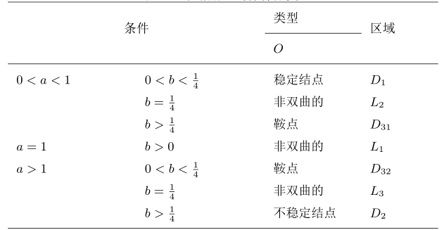
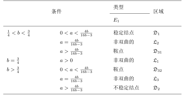
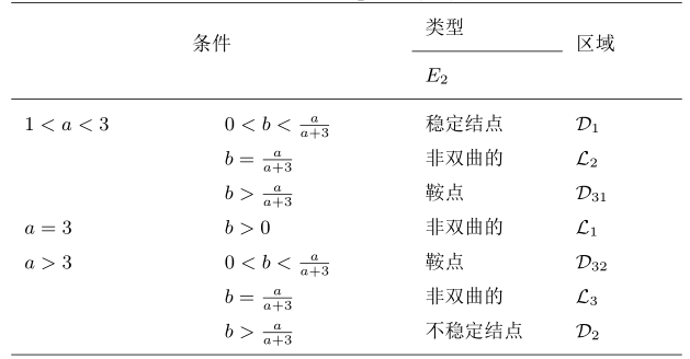
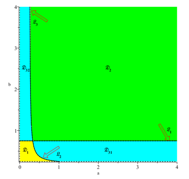
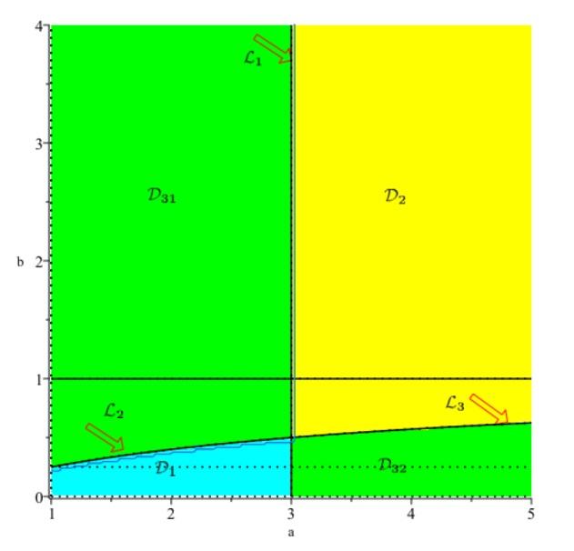
的条件下存在. 进一步, 将 $O,~E_1$及$E_2$的拓扑分类和非双曲情形的参数条件列于表1-3, 相应的参数图如图1-3.

证 系统(2.1)的不动点由方程组

决定, 求解上述二元非线性方程组, 易知系统(2.1)的前三个不动点为

考虑到系统(2.1)中$0\leq x\leq1, 0\leq y\leq1$, 因此$O$总是存在, 而$E_1$存在的条件是$a>0,~b>{1}/{4}$, $E_2$ 在$a>1, ~b>0$ 时存在.

系统(2.1)在不动点$O$, $E_1$, $E_2$处的Jacobian矩阵分别为

显然, $JF(O)$的两个特征值是$a$和$4b$, 因此, 不动点$O$是非双曲的当且仅当$a$或$4b$位于复平面$\mathbb{C}^1$中的单位圆$S^1$上, 也就是$a=1$或$b={1}/{4}$, 除此之外, 不动点$O$是双曲的. 因此, $O$有以下拓扑类型

(i) $0<a<1,~0<b<{1}/{4}$, $O$为稳定结点; (ii) $0<a<1,~b={1}/{4}$, $O$ 为非双曲不动点;

(iii) $0<a<1,~b>{1}/{4}$, $O$为鞍点; (iv) $a=1,~b>0$, $O$ 为非双曲不动点;

(v) $a>1,~0<b<{1}/{4}$, $O$为鞍点; (vi) $a>1,~b={1}/{4}$, $O$ 为非双曲不动点;

(vii) $a>1,~b>{1}/{4}$, $O$为不稳定结点.

往下, 我们讨论不动点$E_1$的定性性质. 矩阵$JF(E_1)$的两个特征值分别是$-4\,b+2$和${a\,(16\,b-3)}/{4\,b}$, 显然这两个特征值均为实数, 而$JF(E_1)$的特征多项式为

进一步, 该特征多项式的判别式为 $ \bigtriangleup({P_{E_1}}(t))=\frac{\left(16 a b+16 b^{2}-3 a-8 b\right)^{2}}{16 b^{2}}\mbox{, } $ 对称轴为 ${t_1}=(16 a b-16 b^{2}$$-3 a+8 b)/{8 b}\mbox{,}$ 于是, 我们有

(i) 若$E_1$是非双曲的, 则${JF(E_1)}$的特征值的模等于$1$. 此时, ${P_{E_1}}(1)=0$, ${P_{E_1}}(-1)=0$, 因此, 相应的非双曲参数条件为

$\bullet$$b>\frac{1}{4},~a=\frac{4\,b}{16\,b-3}$;

$\bullet$$b=\frac{3}{4},~a>0$.

(ii) 若$E_1$是稳定结点, 则$JF(E_1)$的两个特征值都位于单位圆内, 这意味着${P_{E_1}}(1)>0$, ${P_{E_1}}(-1)>0$, ${\bigtriangleup({P_{E_1}}(t))}\geq0$, $-1<{t_1}<1$, 结合$E_{1}$的存在条件, 我们可以得到如下半代数系统

运用多项式完全判别系统理论以及多项式代数系统${\tt Maple 2024}$, 可得上述半代数系统的解集为

(iii) 若$E_1$是不稳定结点, 此时$JF(E_1)$的两个特征值都在单位圆外, 其参数条件满足下列三种情形

$\blacklozenge$${P_{E_1}}(1)<0$, ${P_{E_1}}(-1)<0$, ${\bigtriangleup({P_{E_1}}(t))}>0$;

$\blacklozenge$${P_{E_1}}(1)>0$, ${P_{E_1}}(-1)>0$, ${\bigtriangleup({P_{E_1}}(t))}\geq0 $, ${t_1}<-1$;

$\blacklozenge$${P_{E_1}}(1)>0$, ${P_{E_1}}(-1)>0$, ${\bigtriangleup({P_{E_1}}(t))}\geq0 $, ${t_1}>1$.

运用情形(ii)中同样的方法, 我们可以得到半代数系统${PS_{2}}$, ${PS_{3}}$, ${PS_{4}}$. 进一步, 对${PS_{2}}$, ${PS_{3}}$, ${PS_{4}}$ 进行求解, 可知${PS_{3}}$, ${PS_{4}}$无解, 而$PS_{2}$的解集为

(iv) 若$E_1$是鞍点, 则$JF(E_1)$的特征值一个位于单位圆内, 另一个位于单位圆外, 那么此时参数条件有如下两种情形

$\blacklozenge$${P_{E_1}}(1)<0$, ${P_{E_1}}(-1)>0$, ${\bigtriangleup({P_{E_1}}(t))}>0 $, ${t_1}>-1$;

$\blacklozenge$${P_{E_1}}(1)>0$, ${P_{E_1}}(-1)<0$, ${\bigtriangleup({P_{E_1}}(t))}>0 $, ${t_1}<1$.

类似地, 我们可以得到上述两种情形对应的半代数系统${PS_{5}}$, ${PS_{6}}$. 求解得到

对于不动点$E_{2}$的定性性质. 容易验证, 矩阵$JF(E_2)$的两个特征值是$-a+2$ 和${b\,(a+3)}/{a}$, 这两个特征值都是实数, 而$JF(E_2)$的特征多项式为 $ {P_{E_{2}}}(t)=-\frac{\left(a-2+t\right) \left(\left(b-t\right) a+3 b\right)}{a}\mbox{, } $ 其相应的判别式为 $ \bigtriangleup({P_{E_{2}}}(t))=\frac{\left(a^{2}+b a-2 a+3 b\right)^{2}}{a^{2}}\mbox{, } $ 对称轴为 ${t_2}=-{(a^{2}-b a-2 a-3 b)}/{2 a}\mbox{.}$

(i) 若$E_{2}$是非双曲的, 则${JF(E_{2})}$的特征值的模等于$1$, 那么此时参数条件有两种情形, 分别是${P_{E_{2}}}(1)=0$, ${P_{E_{2}}}(-1)=0$. 进一步, 我们可以求得参数范围为

$\bullet$$a>1, b=\frac{a}{a + 3}$;

$\bullet$$a=3,b>0$.

(ii) 若$E_{2}$是稳定结点, 则$JF(E_{2})$的两个特征值均位于单位圆内, 这意味着${P_{E_{2}}}(1)>0$, ${P_{E_{2}}}(-1)>0$, ${\bigtriangleup({P_{E_{2}}}(t))}\geq0 $, $-1<{t_2}<1$, 结合$E_{2}$ 的存在条件, 我们可以得到如下半代数系统

运用多项式判别理论, 我们可以求得上述半代数系统的解为 $ {{PS_{7}}}=\Big\{(a,b)\Big|1<a<3,0<b<\frac{a}{a+3}\Big\}\mbox{; } $

(iii) 若$E_{2}$是不稳定结点, $JF(E_{2})$的两个特征值都在单位圆外, 其相应的参数条件有如下三种情形, 分别为

$\blacklozenge$${P_{E_{2}}}(1)<0$, ${P_{E_{2}}}(-1)<0$, ${\bigtriangleup({P_{E_{2}}}(t))}>0$;

$\blacklozenge$${P_{E_{2}}}(1)>0$, ${P_{E_{2}}}(-1)>0$, ${\bigtriangleup({P_{E_{2}}}(t))}\geq0 $, ${t_2}<-1$;

$\blacklozenge$${P_{E_{2}}}(1)>0$, ${P_{E_{2}}}(-1)>0$, ${\bigtriangleup({P_{E_{2}}}(t))}\geq0 $, ${t_2}>1\mbox{.}$

设它们对应的半代数系统分别为${PS_{8}}$, ${PS_{9}}$, ${PS_{10}}$. 进一步, 求解以上半代数系统, 我们可以得到${PS_{9}}$, ${PS_{10}}$无解, 而$PS_{8}$的解集为

(iv) 若$E_{2}$是鞍点, 则$JF(E_{2})$的特征值一个位于单位圆内, 另一个位于单位圆外, 那么此时参数条件有下列两种情形, 分别为

$\blacklozenge$${P_{E_{2}}}(1)<0$, ${P_{E_{2}}}(-1)>0$, ${\bigtriangleup({P_{E_{2}}}(t))}>0 $, ${t_2}>-1$;

$\blacklozenge$${P_{E_{2}}}(1)>0$, ${P_{E_{2}}}(-1)<0$, ${\bigtriangleup({P_{E_{2}}}(t))}>0 $, ${t_2}<1\mbox{.}$

同理, 我们可以得到与之对应的两个半代数系统${PS_{11}}$, ${PS_{12}}$. 进一步, 解得

上述证明所得结果已列于表1-3.

注 2.1 经过计算, 我们发现不动点$E_3$的特征值是非代数的且带有多个根号, 无法用现有的代数系统理论对其进行处理, 从而无法给出$E_3$的完整拓扑分类, 因此我们只能考虑$E_3$的稳定性. 系统(2.1)在$E_3$处的Jacobian矩阵可被表示为

其中$\alpha$由命题2.1给出. 其对应的特征多项式为 $ {P_{E_{3}}}(t):= t^2 + \beta_1 t + \beta_2 \mbox{, } $ 其中

由平衡解稳定性理论^[18]知, 二次方程$t^2 + \beta_1 t + \beta_2 = 0$的两个根的模都小于$1$的充分必要条件是

若同时满足以上三个条件, 则平衡解构成汇. 又$E_3$的存在条件为

于是, $E_3$的稳定性可由以下标准确定: 若满足 $ \Lambda: = \Gamma \cap \big\{(a,b)\big|1+\beta_1+\beta_2>0,~1-\beta_1+\beta_2>0,~1-\beta_2>0 \big\} \mbox{,} $ 则$E_3$为汇.

注意到, 受个人计算机的内存所限, 我们无法借助多项式完全判别系统理论及多项式代数系统${\tt Maple 2024}$获得半代数系统$\Gamma$的解集, 而只能给出上述定性表达式.

接下来, 在命题2.1给出的非双曲参数条件下, 我们将应用映射分岔理论^[19]和中心流形定理^[20]讨论不动点$O$, $E_1$和$E_2$的分岔现象.

本节讨论在非双曲情形$a=1$或$b=1/4$下, $O$点的分岔现象.

定理 3.1 当$b>0$时, 系统(2.1)在 $a=1$ 附近发生跨临界分岔. 即, 当$0<b<1/4$时, 在$0<a<1$的情况下, 不动点$O$为稳定结点, $E_2((a-1)/a,0)$没有生物学意义; 在$a=1$的情况下, $O$与$E_2$共存; 在$a>1$的情况下, $O$为鞍点, $E_2$ 为稳定结点.

证 令$\delta :=a-1$, 则$a=\delta+1$, 将系统(2.1)进行Taylor展开, 可得如下扩展形式的映射

易知其Jacobian矩阵$J\Phi_0(O)$有特征向量$(0,0,1)^T$, $(0,1,0)^T$ 和 $(1,0,0)^T$, 分别对应特征值$4b$, $1$, $1$, 即

进一步, 将系统(3.1)的线性部分进行对角化, 我们得到如下映射

由于$J\Phi_0(O)$在单位圆$S^1$上有两个特征值, 根据中心流形定理, 系统(3.2)存在二维${C}^2$中心流形

其中, $h_1$为$(0,0)$附近的${C}^2$函数, 使得

并且$\xi_1$, $\xi_2$都是充分小的正常数. 注意到${C}^2$的光滑性, 我们将$h_1(\nu,\delta)$的形式设为

其中$a_{20}$, $a_{11}$和$a_{02}$为待定常数. 根据中心流形的不变性, 并结合(3.3)和(3.4)式, 我们有 $ h_1(-3 (\delta + 1)(h_1(\nu,\delta) + \frac{1}{3}) \nu (\nu - 1),\delta) =b\, h_1(\nu,\delta) (h_1(\nu,\delta) - 1) (3 \nu - 4) \mbox{, } $ 从而 $ a_{20}\nu^2 +a_{11}\nu \delta +a_{02}\delta^2+O(|(\nu,\delta)|^3)=O(|(\nu,\delta)|^3)\mbox{.} \label{coe1} $ 利用待定系数法, 可得$a_{20}=a_{11}=a_{02}=0$. 结合(3.4)式, 我们有

将(3.5)式代入(3.2)式的后两个方程, 我们得到如下映射

事实上, 上式定义了一个一维映射 $ \nu \mapsto g_{\delta}(\nu):= \nu - \nu^{2} + \nu\delta - \nu^{2}\delta +O(|(\nu,\delta)|^4)\mbox{.} $ 因此

上面的式子表明, 系统(2.1)满足跨临界分岔的非退化性条件和横截性条件^[21]. 因此, 当参数跨过曲线$\{(a,b)|a=1,b>0\}$时, 系统(2.1)发生跨临界分岔.

根据定理3.1的证明, 当$b>0$时, 存在一个1维稳定流形在$O$处与$\omega$轴相切, 一个2维中心流形与平面$\omega=0$(即系统(3.2)中的$(\delta,v)$平面)相切. 跨临界分岔发生在中心流形上, 即在$\delta=0$的两侧, 两个不动点$O$与$E_2$的稳定性发生交换. 同理可得

定理 3.2 当$a>0$时, 系统(2.1)在$b=1/4$ 附近发生跨临界分岔. 即是说, 当$0<a<1$时, 在$0<b<1/4$的情形下, 不动点$O$为稳定结点, $E_1(0,(4b-1)/4b)$没有生物学意义; 在$b=1/4$的情况下, $O$与$E_1$共存; 在$b>1/4$的情况下, $O$为鞍点, $E_1$为稳定结点.

由定理3.1和定理3.2可知, 系统(2.1)在不动点$O$与$E_1$以及$O$与$E_2$处存在一个在稳定和不稳定之间过渡的阈值, 即该阈值设计了一个方案来控制捕食者和食饵的种群数量

(i) 对于$b>0$和$0<a<1$, 如果食饵繁殖力低下, 那么捕食者和食饵的数量将急剧减少, 最终共同灭绝;

(ii) 如果$b>0$和$a>1$, 捕食者的数量在0附近, 食饵繁殖力强且初始数量较少, 那么食饵会突破临界值, 捕食者被淘汰, 食饵稳定存活, 食饵的种群密度稳定于$(a-1)/a$附近;

(iii) 对于$a>0$和$0<b<1/4$, 过低的捕食者繁殖率将阻碍其维持最低生存种群的能力, 造成食饵过度消耗资源并衰退, 继而引发整个系统的持续萎缩和双向灭绝;

(iv) 如果$a>0$和$b>1/4$, 当捕食者内禀增长率显著高于系统承载力, 且食饵初始种群密度低于临界阈值时, 捕食者增长参数与食饵初始数量的失衡将导致相空间轨迹偏离不动点$O$, 使系统沿不稳定流形滑向不动点$E_1(0, (4b-1)/4b)$(即食饵灭绝, 捕食者存活, 捕食者的种群密度稳定于$(4b-1)/4b$附近).

本节考虑讨论$E_1$的非双曲情形, 即$\{(a,b)|1/4<b<3/4,~a=4b/(16b-3)\}$, 或$\{(a,b)|b=3/4,~a>0\}$, 或$\{(a,b)|b>3/4,~a=4 b/(16b-3)\}$. 由于不动点$E_1(0,(4b-1)/4b)$和$E_2((a-1)/a,0)$是形式对称的, 因此$E_2$的非双曲情形可根据$E_1$的非双曲情形得出.

定理 4.1 当$b>1/4$时, 系统(2.1)在跨过曲线$a=4b/(16b-3)$时发生跨临界分岔.

证 令$\delta := a - {4b}/{(16b-3)}$, 则$a= \delta + {4b}/{(16b-3)}$. 如定理3.1的证明一样, 将$E_1$平移到原点$O$, 并将系统(2.1)所示映射$T_{a,b}$限制到二维${C}^2$ 中心流形

由此定义如下一维映射

易知

满足跨临界分岔的非退化性条件和横截性条件, 这意味着当参数跨过曲线$\{(a,b)|b>{1}/{4},a={4 b}/{(16 b-3)}\}$时, 系统(2.1)发生跨临界分岔.

定理4.1证明了当$b>1/4$时, 存在一个1维稳定流形在$E_1$处与$\zeta$轴相切, 一个2维中心流形与平面$\zeta=0$(即$(\delta,\theta)$平面)相切. 跨临界分岔发生在中心流形上, 即在$\delta=0$的两侧, 两个不动点$E_1$与$E_{3}$的稳定性发生交换.

除了非双曲情形$\{(a,b) |\, b>{1}/{4},a={4 b}/{(16 b-3)}\}$, 即矩阵$JF(E_1)$的特征值为$1$外, 系统(2.1)在不动点$E_1$处还存在另一种非双曲情形, 即当$b={3}/{4}$且$a>0$时, 矩阵$JF(E_1)$的特征值为$-1$. 因此, 我们进一步讨论当$(a,b)$跨过曲线$\{(a,b)|\, b={3}/{4},a>0\}$ 时, 系统(2.1)是否会发生翻转分岔.

定理 4.2 当$0<a<4 b/(16 b-3)$, 且参数$(a,b)$从区域$\mathfrak{D}_{1}$到区域$\mathfrak{D}_{32}$跨过曲线$b=3/4$ 时, 系统(2.1)发生超临界翻转分岔, 并在不动点$E_1$ 附近产生稳定的周期二环.

证 令$\delta :=b-{3}/{4}$, 则$b=\delta+{3}/{4}$. 我们首先将系统(2.1)所示映射$T_{a,b}$限制到二维${C}^2$中心流形 $ \zeta=h_3(\theta,\delta)=O(|(\theta,\delta)|^3)\mbox{, } $ 并由此得到相应的一维映射

进一步

以及

和

因此满足文献 [条件(F1)和(F2)]{Guckenheimer83}. 于是, 当$0<a<4 b/(16 b-3)$, 参数$(a,b)$ 穿过曲线$b={3}/{4}$时, 系统(2.1)发生翻转分岔. 从上述证明过程中可以得出, 在曲线$\{(a,b)|\,b={3}/{4}, 0<a<4 b/(16 b-3) \}$邻近的区域$\mathfrak{D}_{32}$ 内, 系统(2.1)发生超临界翻转分岔.

此外, 映射(4.1)在拓扑等价意义下可简化为以下形式

对$\mathcal{F}^{*}_{\delta}$进行关于$\theta$的 Taylor 级数展开, 可得其局部表达式为

其中系数函数$f_1,f_2,f_3\in {C}^1$, 且满足

此处$g$亦为${C}^1$类函数, 且满足初始条件$g(0)=0$.

进一步, 由偏导数条件

可知$g$在$\delta=0$处满足反函数定理条件, 故$g$是局部可逆的. 据此定义新参数 $ \delta_1:=g(\delta)=4 \delta. $ 映射(4.4)可取为如下形式

其中$\mu(\delta_1)=-(1+\delta_1)$, 光滑函数$a(\delta_1)$和$b(\delta_1)$满足初始条件

往下, 我们考虑如下光滑的坐标变换

其中, $\delta_2=\delta_2(\delta_1)$是待定的光滑函数. 变换(4.6)式在原点的某个领域内可逆, 其逆变换由待定系数法确定为

利用(4.6)和(4.7)式, 可将(4.5)式转化为

由条件$\mu^2(0)-\mu(0)=2\neq0$, 对充分小的$\delta_1$, 选择

则二次项就可以被"消去", 进而(4.8)式变换为

其中光滑函数$c(\delta_1)$满足

且由条件(4.2)有$c(0)>0$. 其中, $c(0)$的符号决定了周期二环的稳定性和分岔方向^[22], 即如果$c(0)>0$对应稳定周期二环(发生超临界翻转分岔), 如果$c(0)<0$对应不稳定周期二环(发生亚临界翻转分岔).

通过引入重尺度化变换

在新坐标$\eta$下, 映射(4.4)可转化为

由此, 根据文献[19,定理4.4], 在原点$O$邻域内, 映射(4.9)与如下形式拓扑等价

进一步研究映射(4.10)的二次迭代可得

当$0<\delta_1\ll1$时, $F^2(\eta)$存在一个平凡不动点$\eta_0=0$和两个非平凡的不动点

通过验证$|DF^2(\eta_{1,2})|<1$可知, $\eta_1$和$\eta_2$均为稳定不动点, 构成了原映射$F(\eta)$稳定的周期二环. 这表明当$0 <\delta \ll 1$时, 映射(4.3)在不动点$E_1$附近产生稳定的周期二环. 进一步地, 当参数$(a,b)$位于曲线$\{(a,b) |b={3}/{4},0<a<{4 b}/{(16 b-3)}\}$邻近的区域$\mathfrak{D}_{32}$时, 系统(2.1)存在稳定的周期二环结构.

定理 4.3 在参数满足$a>4 b/(16 b-3)$的条件下, 当$(a,b)$由区域$\mathfrak{D}_{31}$穿越临界曲线$b=3/4$进入区域$\mathfrak{D}_{2}$时, 系统(2.1)发生翻转分岔. 此外, 在该曲线$\{(a,b) |b=3/4,a>4 b/(16 b-3)\}$邻近的区域$\mathfrak{D}_{2}$内, 系统(2.1)经历超临界翻转分岔, 并在不动点$E_1$的邻域中形成稳定的周期二环.

由定理4.2, 4.3可知, 当参数满足$a>0$且$1/4<b<3/4$时, 系统(2.1)的不动点$E_1(0,(4b-1)/4b)$ 是局部渐近稳定的, 此时, 食饵灭绝而捕食者维持于平衡状态. 当参数跨越临界曲线$\{(a,b)|a>0,b=3/4\}$时, 系统(2.1)发生翻转分岔, 使得平衡失稳并出现稳定的周期二环, 表现为捕食者种群密度在高低水平间交替波动. 该现象表明, 在捕食者不完全依赖该食饵物种(如存在其他食物来源)的假设下, 当环境条件发生临界变化时, 即便食饵灭绝, 捕食者种群密度也无法维持在恒定水平, 其内部的密度制约机制将取代种间相互作用, 成为驱动种群动态的主导力量, 使其进入由自身动力决定的周期性振荡.

考虑$E_2$点的非双曲情形, 即$\{ (a,b) |1<a<3,~b=a/(a+3)\}$, 或$\{ (a,b) |a=3,~b>0\}$, 或$\{ (a,b) |a>3,~b=a/(a+3)\}$. 运用定理4.1和4.2中的证明方法可知, 系统(2.1)在曲线$\{(a,b) |1<a<3,~b=a/(a+3)\}$以及$\{(a,b) |a>3,~b=a/(a+3)\}$附近发生跨临界分岔, 在曲线$\{(a,b) |a=3,~b>0\}$附近发生超临界翻转分岔. 于是可得下面的定理

定理 4.4 当$a > 1$时, 系统(2.1)在穿越曲线$b=a/(a+3)$时发生跨临界分岔.

注 4.1 根据注2.1, $E_3$的存在条件由半代数系统$\Gamma$的解集定义. 然而, 由于$\Gamma$的不可解性, 因此$E_3$的存在条件无法判定, 进而导致无法确定$E_1$与$E_3$以及$E_2$与$E_3$不动点间稳定性交换的临界参数条件, 从而无法给出定理4.1与定理4.4的生物学意义解释.

定理 4.5 当$b>0$时, 参数$(a,b)$从区域$\mathcal{D}_{1}$到$\mathcal{D}_{32}$(或从区域$\mathcal{D}_{31}$到$\mathcal{D}_{2}$)跨过曲线$a=3$时, 系统(2.1)发生超临界翻转分岔, 并在不动点$E_2$附近产生稳定的周期二环.

根据定理4.5, 当参数满足 $1 < a < 3$ 且 $b > 0$ 时, 不动点 $E_2((a-1)/a, 0)$ 是局部渐近稳定的, 此时捕食者灭绝, 食饵种群稳定在平衡状态. 当参数越过临界曲线 $\{(a, b) \mid a = 3,\,b > 0\}$ 时, 系统(2.1)发生翻转分岔, 导致该平衡失稳, 并出现一个稳定的周期-2轨道. 此时, 食饵种群密度呈现稳定的周期振荡, 表现为“高-低”交替波动. 这一现象表明, 即使捕食者灭绝, 食饵种群自身的强密度制约效应仍会阻止其趋于平衡, 并在临界参数条件下由种群内部动力主导增长, 从而形成周期性波动.

在讨论系统(2.1)的混沌行为之前, 我们首先引入关于Marotto意义下混沌的基本定义和相关结论[23-25].

不动点$E$称为$f:\mathbb{R}^n \rightarrow \mathbb{R}^n $ 的排斥不动点^[23], 如果对任意$X \in B_r(E)$, $Df(X)$ 的所有特征值的模都大于1, 其中$B_r(E)$是不动点$E$的一个邻域, $f$在$B_r(E)$中可微.

定义 5.1^[24,25] 设$E$是$f$在$B_r(E)$中的一个排斥不动点. 对于某个$r>0$, 若存在一点$x_0\in B_r(E)$且$x_0\ne E$, 使得对于$1\leq k\leq M$, $x_M=E$且$|Df(x_k)|\ne0$, 其中$x_k=f^k(x_0)$, 则称$E$为$f$的回弹排斥子.

引理 5.1^[24,25] 如果$f$有一个回弹排斥子, 则$f$是混沌的.

利用上述结论我们需要验证$O$是系统(2.1)的回弹排斥子. 与不动点$O(0,0)$相关的特征值可由下式给出

其中

令$\mathbf{p_0}$和$\mathbf{q_0}$为$\mathbf{p}, \mathbf{q}$在$O$处的取值, 由于$\mathbf{p_0}^2-4\mathbf{q_0}=\left( a - 4b \right)^{2}\geq0$, 于是存在$O$的一个邻域$\mathcal{I}_1$, 使得对任意$(x,y)\in \mathcal{I}_1$, $\mathbf{p}^2(x,y)-4\mathbf{q}(x,y)\geq0$恒成立. 由定义5.1可知, 我们只需要验证$O(0,0)$满足如下条件之一

(i) $\mathbf{p}(0,0)\leq 0, 1-\mathbf{p}(0,0)+\mathbf{q}(0,0)<0$;

(ii) $\mathbf{p}(0,0)>0, 1+\mathbf{p}(0,0)+\mathbf{q}(0,0)<0$;

(iii) $\mathbf{p}(0,0)<-2, 1+\mathbf{p}(0,0)+\mathbf{q}(0,0)>0,\mathbf{p}^2(0,0)-4\mathbf{q}(0,0)\geq 0$;

(iv) $\mathbf{p}(0,0)>2, 1-\mathbf{p}(0,0)+\mathbf{q}(0,0)>0,\mathbf{p}^2(0,0)-4\mathbf{q}(0,0)\geq 0$.

这等价于$O$的两个特征值的模均大于1, 即$|a|>1, |4 b|>1$. 结合$O$的存在条件(即$a>0,b>0$), 我们可得当$a>1,b>{1}/{4}$时, $O$的两个特征值的模恒大于1. 于是, 存在$O$的一个邻域$\mathcal{I}_2$, 使得对任意$(x,y)\in \mathcal{I}_2$, 有$|\lambda^0_{1,2}|>1$成立. 进一步地, 我们通过$\mathcal{I}_0 := \mathcal{I}_1 \cap \mathcal{I}_2$得到一个新邻域$\mathcal{I}_0$, 使得对于任意$(x,y)\in \mathcal{I}_0$, $\mathbf{p}^2(x,y)-4\mathbf{q}(x,y)\geq0$ 以及 $|\lambda^0_{1,2}|>1$均成立, 从而$\mathcal{I}_0$就是定义5.1中所要找的$B_r(O)$.

根据回弹排斥子的定义, 下面我们需要在$\mathcal{I}_0$中找一点$z_0$, 使得对于任意的$1\leq k\leq M$, $z_M=O$且${\det} (JF(z_k)) \ne 0$, 其中$z_k=f^k(z_0)$.

事实上, 根据系统(2.1)可知

和

直接计算可知, 方程(5.4)的其中一个非零解为$(x'',y'')=(0,1)$, 将其代入方程(5.3)求解, 可得一个非零解为$(x',y')=(0,{(b-\sqrt{b^{2}-b})}/{2 b})$, 其中$b>1$. 进一步, 设$O$的某一个$k \in \mathbb{N}^{+}$次原像为$(0,y_k)$, 令$y_{k+1}={(b-\sqrt{b^{2}-y_{k}})}/{2 b}$, 我们将说明存在$K \in \mathbb{N}^{+}$, 使得$y_K$位于$\mathcal{I}_0$中.

首先, 通过归纳法可知, $y_k$的极限是存在的. 其次, 通过方程$y_{k+1}={(b-\sqrt{b^{2}-y_{k}})}/{2 b}$, 可得$\lim_{k\rightarrow\infty}y_k = 0$. 因此, 存在$K\in\mathbb{N}^{+}$, 使得对于任意的$k \geq K$, $y_k$位于$\mathcal{I}_0$中. 于是, 令$z_0:=(0,y_K)$. 系统(2.1)在$z_k$处的Jacobian矩阵为

于是${\det} (JF(z_k))=- 4 a b \left(3 y_k+1\right) \left(2 y_k-1\right)$. 考虑到在$\mathcal{I}_0$中, $a>1$, $b>{1}/{4}$, 从上述分析可知$y_k \neq {1}/{2}$. 因此, 对于任意的$1 \leq k \leq M$, ${\det} (JF(z_k)) \ne 0$, 于是$O$是一个回弹排斥子. 根据引理5.1可知, 系统(2.1)存在Marotto意义下混沌. 综上所述, 我们可以得出以下结论:

定理 5.1 若$(x,y)\in \mathcal{I}_0$, 且方程(5.3)和(5.4)的实零点不同于$O$, 即$(x',y')$, $(x'',y'')\ne (0,0)$, 并且对于任意的$1\leq k\leq M$, ${\det} (JF(z_k))\ne0$, 则$O$是系统(2.1)的一个回弹排斥子, 因此系统(2.1)具有Marotto意义下的混沌.

其次, 说明$E_1$也是系统(2.1)的回弹排斥子. 类似地, 当$b>{3}/{4},a>{4 b}/{(16 b-3)}$时, $E_1$的两个特征值的模均大于$1$. 因此, 存在$E_1$的一个邻域$\mathfrak{I}_0$, 即为定义5.1所求的$B_r(E_1)$, 使得对所有$(x,y)\in \mathfrak{I}_0$, 不等式 $\mathbf{p}^2(x,y)-4\mathbf{q}(x,y)\geq0$ 及$ |\lambda^1_{1,2}| > 1$同时成立, 这里$\mathbf{p}(x,y)$和$\mathbf{q}(x,y)$定义见(5.1)和(5.2)式, 而$\lambda^1_{1,2}$是与$E_1$相关的两个特征值. 进一步, 为满足回弹排斥子的定义, 我们还需在$\mathfrak{I}_0$ 中选取一点$z_0$, 使得对所有的$1\leq k\leq M$, 迭代轨道$\{z_k=f^k(z_0)\}$满足$z_M=E_1$, 且Jacobian矩阵行列式$\mathit{\det} (JF(z_k)) \ne 0$.

实际上, 通过系统(2.1)分析可知, $E_1(0,(4b-1)/4b)$ 的一个原像为$(x'',y'')=(0,{1}/{4 b})$, 进一步推导可得, 与$(x'',y'')$对应的一个原像为$(x',y')=(0,{(2 b+\sqrt{4 b^{2}-1})}/{4 b})$, 其中$b>1/2$. 现假设$E_1$的某个$k \in \mathbb{N}^{+}$次原像为$(0,y_k)$, 并定义递推关系$y_{k+1}={(2 b+\sqrt{\left(4 b y_{k}-2 b\right) \left(2 b-1\right)})}/{4 b}$. 接下来我们将指出存在正整数$K$, 使得$y_K$属于邻域$\mathfrak{I}_0$.

根据数学归纳法, 序列$y_k$的极限存在且收敛于${(4 b-1)}/{4 b}$(即$E_1$的纵坐标). 因此, 存在正整数$K$, 使得对所有$k \geq K$, 点$(0,y_k)$位于$E_1$的排斥邻域$\mathfrak{I}_0$内. 令初始点$z_0:=(0,y_K)$, 迭代序列$z_k=f^k(z_0)$满足$z_M=E_1$. 而系统(2.1)在$z_k$处的Jacobian矩阵的行列式为${\det} (JF(z_k))=- 4 a b \left(3 y_k+1\right) \left(2 y_k-1\right) $, 并且在邻域$\mathfrak{I}_0$内, 参数满足$ b>{3}/{4},\,a>{4 b}/{(16 b-3)}$, 由上述分析可得$y_k \neq {1}/{2}$, 从而${\det} (JF(z_k)) \ne 0$对所有的$1 \leq k \leq M$成立. 因此, $E_1$是一个回弹排斥子, 根据引理5.1, 系统(2.1)存在Marotto混沌. 据此, 我们可以得出以下结论.

定理 5.2 若$(x,y)\in \mathfrak{I}_0$, 满足$(x',y')$, $(x'',y'') \ne (0,(4b-1)/4b)$, 且对于任意的$1\leq k\leq M$, $\mathit{\det} (JF(z_k))\ne0$, 则$E_1$是系统(2.1)的一个回弹排斥子, 进而系统(2.1)存在Marotto意义下的混沌.

最后, 我们分析$E_{2}$是否为系统(2.1)的回弹排斥子. 采用与前述不动点类似的分析方法, 当参数满足$a>3$且$b > {a}/{(a+3)}$时, $E_2$对应的两个特征值$\lambda^2_{1,2}$的模均大于1. 由此可知, 存在$E_2$的一个邻域$\mathfrak{M}_0$, 使得对于该邻域内任意点$(x,y)$, 不等式$\mathbf{p}^2(x,y) - 4\mathbf{q}(x,y) \geq 0$成立, 且$|\lambda^2_{1,2}| > 1$. 因此, $\mathfrak{M}_0$符合定义5.1中回弹排斥子邻域$B_r(E_2)$的要求.

进一步, 根据回弹排斥子的定义, 我们需要在邻域$\mathfrak{M}_0$内选取点$z_0$, 使得对所有$1 \leq k \leq M$满足$z_M = E_2$且$\det(JF(z_k)) \neq 0$, 其中$z_k = f^k(z_0)$.

实际上, 系统(2.1)经过两次迭代后, $E_2((a-1)/a,0)$ 的一次原像和二次原像分别为$(x'',y'') = (1/a, 0)$与$(x',y') = \left( (a + \sqrt{a^2 - 4})/2a, 0 \right)$, 其中$a > 2$. 设$E_2$的某$k \in \mathbb{N}^{+}$次原像为$(x_k, 0)$, 令$x_{k+1}=(a+\sqrt{(a x_k - 1)(a - 2)})/2a$, 容易验证$\lim_{k \to \infty} x_k = (a-1)/a$(即$E_2$的横坐标). 因此存在正整数$K$, 当$k \geq K$时, $x_k \in \mathfrak{M}_0$. 于是, 令$z_0 := (x_K, 0)$. 系统(2.1)在$z_k$处的Jacobian矩阵为

其行列式为$\det(JF(z_k)) = ab (2x_k - 1)(3x_k - 4)$. 由于在$\mathfrak{M}_0$内, $a > 3$, $b > a/(a+3)$, 经过上述分析可知$x_k \neq 1/2$ 且$x_k \neq 4/3$, 因此, 对所有的$1 \leq k \leq M$ 有$\det(JF(z_k)) \neq 0$, 从而$E_2$为回弹排斥子. 根据引理5.1,系统(2.1)存在Marotto混沌. 由此可得结论

定理 5.3 若$(x,y)\in \mathfrak{M}_0$, 满足$(x',y')$, $(x'',y'') \ne ((a-1)/a,0)$, 且对于任意的$1\leq k\leq M$, ${\det} (JF(z_k)) \ne 0$, 则$E_2$是系统(2.1)的一个回弹排斥子, 从而系统(2.1)具有Marotto意义下的混沌.

根据定理5.1、5.2和5.3可知, 系统(2.1)在Marotto意义下是混沌的, 反映出该捕食者-食饵模型具有显著的非线性与内在复杂性. 该系统对初始种群密度高度敏感, 微小的初始差异会导致长期演化轨迹出现显著分歧: 短期可能呈现周期性振荡, 而长期行为则趋于非周期且不可预测. 尽管系统存在理论上的平衡点, 实际种群动态却可能持续偏离平衡, 表现出固有的不稳定性. 从更深入的视角看, 此类混沌行为揭示了确定性非线性机制主导的生态系统往往遵循某种分形结构演化, 呈现永不重复的确定性波动, 从而排斥传统的平衡态或简单周期模式的描述.

本节将借助${\tt Maple 2024}$和${\tt Matlab R2024a}$对系统(2.1)的动力学行为进行数值模拟, 进而验证第四、五节的理论结果的正确性.

第四节的分析表明, 当参数$a>0$时, 系统$(2.1)$在不动点$E_1$附近会随着参数$b$穿越曲线$b={3}/{4}$而发生超临界翻转分岔. 为此, 我们选择$b$作为分岔参数, 选取特定的$a$ 值进行模拟分析. 取$a=0.2$, 初始点$(x_0, y_0) = (0.01, 0.6)$, 利用${\tt Maple 2024}$绘制出系统$(2.1)$在$(x, y, b)$ 空间上的分岔图6. 从图6可观察到, 当$b$值大于$0.9$时, 系统状态呈现混沌特征. 为验证这一现象, 在${\tt Matlab R2024a}$中计算相应的Lyapunov指数(结果见图6). 从图6可知, 系统的Lyapunov指数在$b = 0.9$ 附近首次转为正值. 该结果与分岔图的观察相符, 即当$b>0.9$时系统$(2.1)$处于混沌状态.

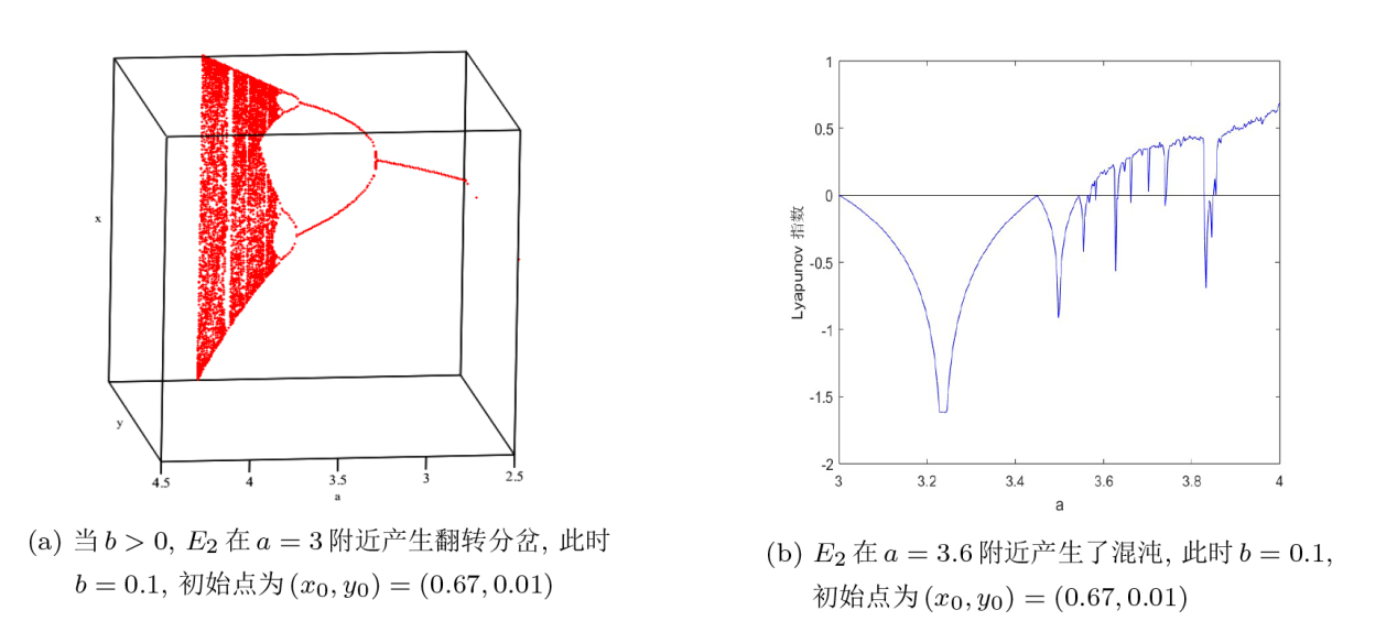
根据第四节的结论, 当$b>0$时, 系统$(2.1)$在不动点$E_2$附近当参数$a$穿越曲线$a=3$时发生超临界翻转分岔. 为此, 选取$a$作为分岔参数, 固定$b=0.1$, 设置初始点$(x_0, y_0) = (0.67, 0.01)$, 通过${\tt Maple 2024}$得到系统$(2.1)$在$(x, y, a)$空间上的分岔图(见图6). 该图显示, 当$a>3.6$时, 系统表现出混沌行为. 为验证这一结果, 使用${\tt Matlab R2024a}$绘制相应的Lyapunov指数图(见图6). 图中可见Lyapunov指数在$a = 3.6$ 附近首次越过零值变为正数. 这与分岔图的观察一致, 由此说明当$a>3.6$时系统$(2.1)$进入混沌状态.

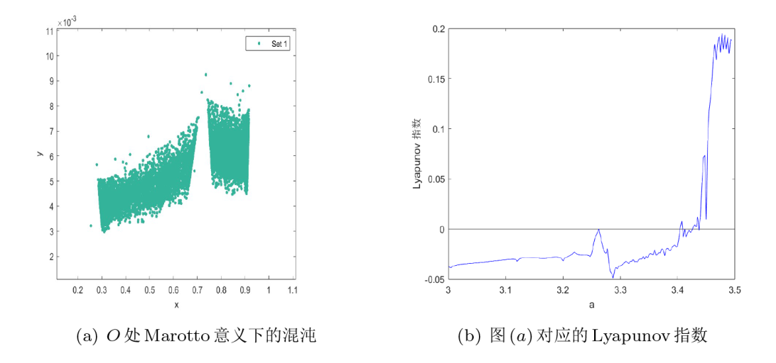
第五节中, 我们验证了$O$, $E_1$, $E_2$均为系统(2.1)的回弹排斥子, 由此表明该系统在Marotto意义下存在混沌现象. 下面, 我们运用${\tt Matlab R2024a}$对系统(2.1)在Marotto意义下的混沌现象进行数值模拟. 首先, 验证系统(2.1)在$O$附近的混沌行为. 依据定理5.1中的条件, 设定参数$a=3.5977$, $b=0.52$, 此时$O$处Jacobian矩阵的特征值$t_1=2.08$与$t_2=3.5977$, 满足$|t_{1,2}|>1$. 选取初始点$(x_0,y_0)=(0.00001,0.00001)$, 根据定理5.1, 此时存在$O$的一个邻域$U_0=\{(x,y)|0.25<x<0.95,0.002<y<0.009\} \subset \mathcal{I}_0$, $O$在$U_0$中具有扩张性. 其二次原像点$O'(x',y')=(0, 0.5 - 0.4803844614 i)$, 满足$T^2_{a,b}(O')=O$且$|DT^2_{a,b}(O')|=621.0088317 \neq 0$. 这就验证了$O$为回弹排斥子, 从而系统(2.1)在$O$附近具有Marotto意义下的混沌. 图6(a)与图6(b)分别展示了$O$附近的混沌现象及对应的Lyapunov指数.

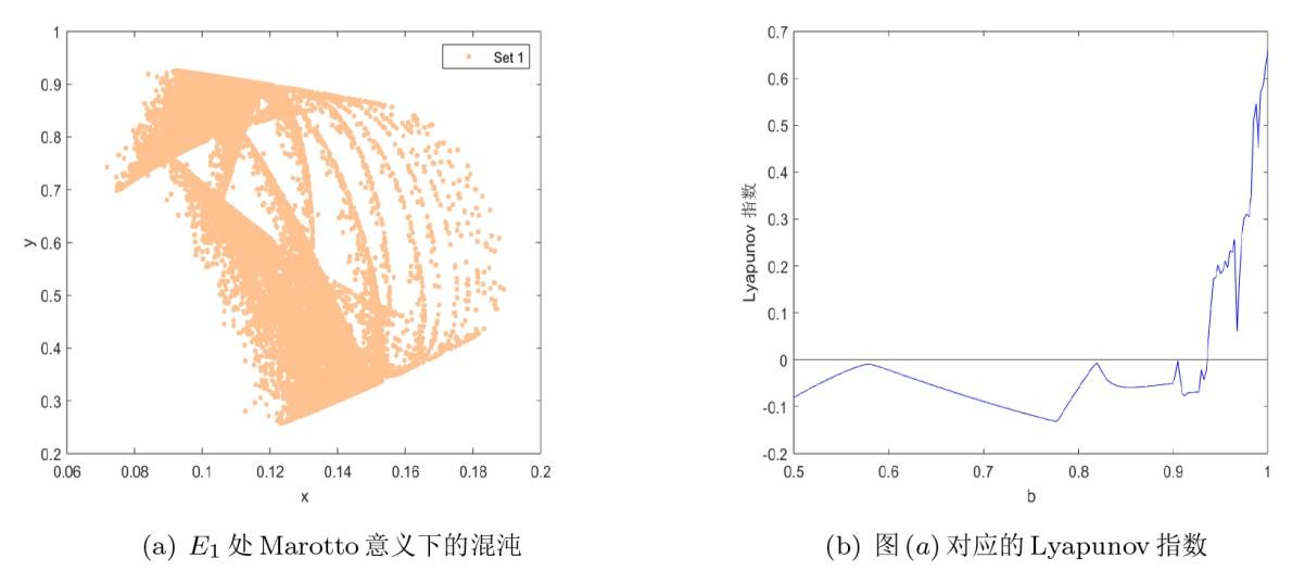
同理, 我们对系统(2.1)在$E_1$附近的Marotto混沌进行数值模拟. 依据定理5.2的条件, 取定参数$a=0.39$, $b=1.005$, 此时系统(2.1)有不动点$E_1(0, 0.7512437811)$. 与其相关的Jacobian矩阵的特征值为$t_1=-2.02$, $t_2=1.268955224$, 且满足$|t_{1,2}|>1$. 选取初始点$(x_0,y_0)=(0.084,0.919)$, 此时可以找到$E_1$的一个邻域$U_1=\{(x,y)|0.065<x<0.195,0.25<y<0.95\} \subset \mathfrak{I}_0$, $E_1$在$U_1$内具有扩张性. 其二次原像点$E_1'(x',y')=(0,0.9337284214)$, 满足$T^2_{a,b}(E_1')=E_1$且$|DT^2_{a,b}(E_1')|=7.11188292 \neq 0$. 由此得出$E_1$是一个回弹排斥子, 进而系统(2.1)存在Marotto混沌. 系统(2.1)在$E_1$附近的混沌行为与对应的Lyapunov指数分别如图7(a)与图7(b)所示.

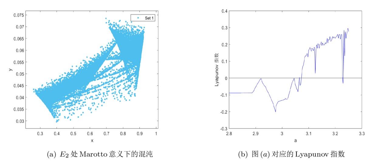
最后, 对系统(2.1)在$E_2$处的混沌行为进行验证. 基于定理5.3的条件, 选定参数$a=3.2$, $b=0.55$, 从而不动点$E_2$的坐标为$(0.6875, 0)$. 该点处Jacobian矩阵的特征值是$t_1 = -1.2$和$t_2 = 1.065625$, 满足$|t_{1,2}| > 1$. 选取初始点$ (x_0,y_0)=(0.813, 0.064)$, 进而可以确定$E_2$的一个邻域$U_2 = \{(x, y) \mid 0.25 < x < 0.95, 0.025 < y < 0.075\} \subset \mathfrak{M}_0$, $E_2$在$U_2$内扩张, 且二次原像点$E_2'(x',y')=(0.8903123748, 0)$, 使得$T^2_{a, b}(E_2')= E_2$, $|DT^2_{a, b}(E_2')| = 3.690799 \neq 0$. 因而, $E_2$构成一个回弹排斥子, 表明系统(2.1)在Marotto意义下存在混沌现象. 此时, 系统(2.1)在$E_2$附近的Marotto混沌现象如图8(a)对应的Lyapunov指数如图8(b).