1 引言
近年来, 基于网络传染病模型的随机动力学研究受到关注 [1 4] . Dangerfield 等 [1 ] 利用扩散近似, 研究了空间结构和随机性在 SIS 型传染病传播中的影响. Graham 和 House[2 ] 探究了异质网络上 SIR 型传染病在早期指数增长阶段的渐近方差. Ball 等 [3 ] 给出了异质网络上 SIR 型传染病的最终规模. Achterberg 和 Van Mieghem[4 ] 推导了广义自适应网络上马尔可夫 SIS 模型的平均场近似. 然而, 关于一般异质网络上传播过程的拟平稳分布的研究仍为有限.
研究拟平稳分布常用的方法之一是矩封闭近似 [5 9] , 即通过系统状态分布的矩来研究传染病传播中的变异性[10 ,11 ] . 一般而言, 矩方程是无限维的, 无法直接处理. 因此, 需要给定分布, 利用该分布矩之间的关系对方程组进行截断, 以获得低阶矩方程. 现有研究在均匀混合层面上评估了给定分布在矩封闭方法上的近似效果, 忽略了传播过程中个体异质性. 本文将该方法推广到异质网络上, 假设传播过程处于阈值之上 (即 $R_{0}>1$ ) , 研究传染病的随机动力学行为.
针对异质网络上 SIS 过程, 本文在第 2 节推导了其 Kolmogorov 微分方程, 并给出了母函数的偏微分方程, 进而得到了过程状态各阶矩的微分方程. 在第 3 节中, 基于正态和对数正态假设, 推导了两组微分方程系统, 并给出了该过程的拟平稳分布和灭绝时间. 在第 4 节中, 借助数值模拟验证了近似的有效性. 最后, 第 5 节给出了结论.
2 SIS网络模型
假设网络为 $N$ $\beta$ $\gamma$
2.1 随机模型
设 $I_{k}(t)$ $S_{k}(t)$ $t$ $k$
$N_{k}$ $k$ $I(t)=(I_{1}(t),I_{2}(t),\cdots,I_{K}(t))$ $K$ $\left\{I(t)\right\}$
当 $\left(i_{1},\cdots,i_{k},\cdots,i_{K}\right)\notin C$ $p_{i_{1},\cdots,i_{k},\cdots,i_{K}}(t)=0$ . 对 $k=1,\cdots,K$ 表 1 列出了度为 $k$ $\mu_{D}$
根据文献[12 ], 前向 Kolmogorov 微分方程如下
(2.1) $\begin{equation}\label{EQ2.1} \begin{aligned} \frac{ p_{i_{1},\cdots,i_{k},\cdots,i_{K}}(t)}{\text{d}t}=&\sum_{k=1}^{K}\biggl\{\beta k[N_{k}-(i_{k}-1)]\frac{\sum_{l\neq k}li_{l}+k(i_{k}-1)}{\mu_{D}N}p_{i_{1},\cdots,i_{k}-1,\cdots,i_{K}}(t)\\ &-\beta k(N_{k}-i_{k})\frac{\sum_{l}li_{l}}{\mu_{D}N}p_{i_{1},\cdots,i_{k},\cdots,i_{K}}(t)\\ &+\gamma(i_{k}+1)p_{i_{1},\cdots,i_{k}+1,\cdots,i_{K}}(t)-\gamma i_{k}p_{i_{1},\cdots,i_{k},\cdots,i_{K}}(t)\biggr\}. \end{aligned} \end{equation} $
下面分析传染病灭绝前的演化过程. 令 $I(t)=\sum_{k=1}^{K}I_{k}(t)$ . 记条件概率为 $q_{i_{1},\cdots,i_{k},\cdots,i_{K}}(t)$
(2.2) $\begin{equation}\label{EQ2.2} \begin{aligned} q_{i_{1},\cdots,i_{k},\cdots,i_{K}}(t)={}&\left\{I_{1}(t)=i_{1},\cdots,I_{k}(t)=i_{k},\cdots,I_{K}(t)=i_{K}\mid I(t)>0\right\}\\ ={}&\frac{p_{i_{1},\cdots,i_{k},\cdots,i_{K}}(t)}{1-p_{0,\cdots,0,\cdots,0}(t)}, \end{aligned} \end{equation}$
$(i_{1},\cdots,i_{k},\cdots,i_{K})\in C\setminus \big\{(0,\cdots,0,\cdots,0)\big\}$ . 基于 (2.1) 式,
(2.3) $\begin{equation}\label{EQ2.3} \begin{aligned} \frac{p_{0,\cdots,0,\cdots,0}(t)}{\text{d}t}=\sum_{k=1}^{K}\gamma p_{e_{k}}(t), \end{aligned} \end{equation}$
其中 $p_{e_{k}}(t)=\mathrm{P}\{I_{1}(t)=0,\cdots,I_{k}(t)=1,\cdots,I_{K}(t)=0\}.$
对 (2.2) 式中的 $q_{i_{1},\cdots,i_{k},\cdots,i_{K}}(t)$
其中 $q_{e_{k}}(t)=\mathrm{P}\left\{I_{1}(t)=0,\cdots,I_{k}(t)=1,\cdots,I_{K}(t)=0\mid I(t)>0\right\}.$
(2.4) $\begin{equation}\label{EQ2.4} \begin{aligned} \frac{q_{i_{1},\cdots,i_{k},\cdots,i_{K}}(t)}{\text{d}t}=&\sum_{k=1}^{K}\biggl\{\beta k[N_{k}-(i_{k}-1)] \frac{\sum_{l\neq k}li_{l}+k(i_{k}-1)}{\mu_{D}N}q_{i_{1},\cdots,i_{k}-1,\cdots,i_{K}}(t)\\ &-\beta k(N_{k}-i_{k})\frac{\sum_{l}li_{l}}{\mu_{D}N}q_{i_{1},\cdots,i_{k},\cdots,i_{K}}(t) +\gamma(i_{k}+1)q_{i_{1},\cdots,i_{k}+1,\cdots,i_{K}}(t)\\ &-\gamma i_{k}q_{i_{1},\cdots,i_{k},\cdots,i_{K}}(t)\biggr\} +\gamma q_{i_{1},\cdots,i_{k},\cdots,i_{K}}(t)\sum_{k=1}^{K}q_{e_{k}}(t). \end{aligned} \end{equation}$
2.2 矩方程
下面给出 $I_{k}\,(k=1,\cdots,K)$ $I_{k}\,(k=1,\cdots,K)$ $M(u_{1},\cdots,u_{k},\cdots,u_{K},t)$
其中 $q_{0,\cdots,0,\cdots,0}(t)=0$ . 使用 (2.4) 式, 得
累积母函数 $G(u_{1},\cdots,u_{k},\cdots,u_{K},t)=\ln M(u_{1},\cdots,u_{k},\cdots,u_{K},t)$
(2.5) $\begin{equation}\label{EQ2.8} \begin{aligned} \frac{\partial G}{\partial t}=&\sum_{k=1}^{K}\frac{\beta kN_{k}}{\mu_{D}N}(e^{u_{k}}-1)\sum_{l=1}^{K}l\frac{\partial G}{\partial u_{l}} -\sum_{k=1}^{K}\frac{\beta k}{\mu_{D}N}(e^{u_{k}}-1)\sum_{l=1}^{K}l\left(\frac{\partial^{2} G}{\partial u_{k}\partial u_{l}} +\frac{\partial G}{\partial u_{k}}\frac{\partial G}{\partial u_{l}}\right)\\[6pt] &+\sum_{k=1}^{K}\gamma(e^{-u_{k}}-1)\frac{\partial G}{\partial u_{k}} +\gamma(1-e^{-G})\sum_{k=1}^{K}q_{e_{k}}. \end{aligned} \end{equation}$
$l,m,n=1,\cdots,K$ $T_{I_{l}I_{m}I_{n}}$ $T_{I_{m}I_{n}^{2}}$
因此, $I_{m}\,(m=1,\cdots,K)$ $I_{m}\,(m=1,\cdots,K)$
(2.6) $\begin{equation}\label{EQ2.9} \begin{aligned} \frac{\text{d} E(I_{m})}{\text{d}t}={}&\frac{\beta m}{\mu_{D}N}\left[N_{m}-E(I_{m})\right]\sum_{l=1}^{K}lE(I_{l}) -\frac{\beta m}{\mu_{D}N}\sum_{l=1}^{K}l\text{Cov}(I_{l},I_{m})\\[4pt] &-\gamma E(I_{m})+\gamma E(I_{m})\sum_{l=1}^{K}q_{e_{l}},\\[4pt] \frac{\text{dVar}(I_{m})}{\text{d}t}={}&\frac{\beta m}{\mu_{D}N}\left[N_{m}-E(I_{m})\right]\sum_{l=1}^{K}lE(I_{l}) +\frac{2\beta m}{\mu_{D}N}\left[N_{m}-E(I_{m})\right]\sum_{l=1}^{K}l\text{Cov}(I_{l},I_{m})\\[4pt] &-\frac{\beta m}{\mu_{D}N}\sum_{l=1}^{K}l\text{Cov}(I_{l},I_{m}) -\frac{2\beta m}{\mu_{D}N}\text{Var}(I_{m})\sum_{l=1}^{K}lE(I_{l}) -\frac{2\beta m}{\mu_{D}N}\sum_{l=1}^{K}lT_{I_{l}I_{m}^{2}}\\[4pt] &+\gamma E(I_{m})-2\gamma\text{Var}(I_{m}) -\gamma E(I_{m})^{2}\sum_{l=1}^{K}q_{e_{l}} +\gamma\text{Var}(I_{m})\sum_{l=1}^{K}q_{e_{l}},\\[4pt] \frac{\text{dCov}(I_{m},I_{n})}{\text{d}t}={}&\frac{\beta m}{\mu_{D}N}\left[N_{m}-E(I_{m})\right]\sum_{l=1}^{K}l\text{Cov}(I_{l},I_{n}) +\frac{\beta n}{\mu_{D}N}\left[N_{n}-E(I_{n})\right]\sum_{l=1}^{K}l\text{Cov}(I_{l},I_{m})\qquad\qquad\qquad\qquad\quad\\[4pt] &-\frac{\beta(m+n)}{\mu_{D}N}\text{Cov}(I_{m},I_{n})\sum_{l=1}^{K}lE(I_{l}) -\frac{\beta(m+n)}{\mu_{D}N}\sum_{l=1}^{K}lT_{I_{l}I_{m}I_{n}}\\[4pt] &-2\gamma \text{Cov}(I_{m},I_{n})-\gamma E(I_{m})E(I_{n})\sum_{l=1}^{K}q_{e_{l}} +\gamma \text{Cov}(I_{m},I_{n})\sum_{l=1}^{K}q_{e_{l}}, \end{aligned} \end{equation}$
根据文献[13 ,14 ], 可知 $R_{0}=\beta(\sigma^{2}_{D}+\mu^{2}_{D})/(\gamma\mu_{D})$ $\sigma^{2}_{D}$ 5 ,15 ], 当 $R_{0}>1$ $q_{e_{l}}\,(l=1,\cdots,K)$ $q_{e_{l}}(t)\,(l=1,\cdots,K)$
(2.7) $\begin{equation}\label{EQ2.10} \begin{aligned} \frac{\text{d}E(I_{m})}{\text{d}t}={}&\frac{\beta m}{\mu_{D}N}\left[N_{m}-E(I_{m})\right]\sum_{l=1}^{K}lE(I_{l}) -\frac{\beta m}{\mu_{D}N}\sum_{l=1}^{K}l\text{Cov}(I_{l},I_{m})-\gamma E(I_{m}),\\[4pt] \frac{\text{dVar}(I_{m})}{\text{d}t}={}&\frac{\beta m}{\mu_{D}N}\left[N_{m}-E(I_{m})\right]\sum_{l=1}^{K}lE(I_{l}) +\frac{2\beta m}{\mu_{D}N}\left[N_{m}-E(I_{m})\right]\sum_{l=1}^{K}l\text{Cov}(I_{l},I_{m})\\[4pt] &-\frac{\beta m}{\mu_{D}N}\sum_{l=1}^{K}l\text{Cov}(I_{l},I_{m}) -\frac{2\beta m}{\mu_{D}N}\text{Var}(I_{m})\sum_{l=1}^{K}lE(I_{l})\\[4pt] &-\frac{2\beta m}{\mu_{D}N}\sum_{l=1}^{K}lT_{I_{l}I_{m}^{2}} +\gamma E(I_{m})-2\gamma \text{Var}(I_{m}),\\[4pt] \frac{\text{dCov}(I_{m},I_{n})}{\text{d}t}={}&\frac{\beta m}{\mu_{D}N}\left[N_{m}-E(I_{m})\right]\sum_{l=1}^{K}l\text{Cov}(I_{l},I_{n}) +\frac{\beta n}{\mu_{D}N}\left[N_{n}-E(I_{n})\right]\sum_{l=1}^{K}l\text{Cov}(I_{l},I_{m})\\[4pt] &-\frac{\beta(m+n)}{\mu_{D}N}\text{Cov}(I_{m},I_{n})\sum_{l=1}^{K}lE(I_{l}) -\frac{\beta(m+n)}{\mu_{D}N}\sum_{l=1}^{K}lT_{I_{l}I_{m}I_{n}}\\[4pt] &-2\gamma \text{Cov}(I_{m},I_{n}), \end{aligned} \end{equation}$
3 拟平稳分布和灭绝时间
由系统 (2.7) 可知, 低阶矩方程包含高阶矩. 为了封闭系统, 使用一阶矩和二阶矩近似三阶矩. 首先, 假设 SIS 传播过程服从多元正态分布, 即 $T_{I_{l}I_{m}I_{n}}=T_{I_{l}I_{m}^{2}}=0~(l,m,n=1,\cdots,K)$ . 因此, 系统 (2.7) 为
(3.1) $\begin{equation}\label{EQ3.1} \begin{aligned} \frac{\text{d}E(I_{m})}{\text{d}t}={}&\frac{\beta m}{\mu_{D}N}\left[N_{m}-E(I_{m})\right]\sum_{l=1}^{K}lE(I_{l}) -\frac{\beta m}{\mu_{D}N}\sum_{l=1}^{K}l\text{Cov}(I_{l},I_{m})-\gamma E(I_{m}),\\ \frac{\text{dVar}(I_{m})}{\text{d}t}={}&\frac{\beta m}{\mu_{D}N}\left[N_{m}-E(I_{m})\right]\sum_{l=1}^{K}lE(I_{l}) +\frac{2\beta m}{\mu_{D}N}\left[N_{m}-E(I_{m})\right]\sum_{l=1}^{K}l\text{Cov}(I_{l},I_{m})\\ &-\frac{\beta m}{\mu_{D}N}\sum_{l=1}^{K}l\text{Cov}(I_{l},I_{m}) -\frac{2\beta m}{\mu_{D}N}\text{Var}(I_{m})\sum_{l=1}^{K}lE(I_{l}) +\gamma E(I_{m})-2\gamma \text{Var}(I_{m}),\\ \frac{\text{dCov}(I_{m},I_{n})}{\text{d}t}={}&\frac{\beta m}{\mu_{D}N}\left[N_{m}-E(I_{m})\right]\sum_{l=1}^{K}l\text{Cov}(I_{l},I_{n}) +\frac{\beta n}{\mu_{D}N}\left[N_{n}-E(I_{n})\right]\sum_{l=1}^{K}l\text{Cov}(I_{l},I_{m})\\ &-\frac{\beta(m+n)}{\mu_{D}N}\text{Cov}(I_{m},I_{n})\sum_{l=1}^{K}lE(I_{l}) -2\gamma \text{Cov}(I_{m},I_{n}), \end{aligned} \end{equation}$
其次, 假设 SIS 传播过程服从多元对数正态分布. 在正态分布下, 各阶矩通过加法联系起来, 即加法矩. 而在对数正态假设下, 这些关系遵循乘法规则. 因此, 采用乘法矩而非加法矩的形式, 矩方程可以用 $\hat{V}_{I_{m}}\,(m=1,\cdots,K)$ $\xi_{I_{m},I_{n}}\,(m,n=1,\cdots,K)$
$l,m,n=1,\cdots,K$ . 使用文献[16 ,17 ], $\hat{T}_{I_{l}I_{m}I_{n}}=\hat{T}_{I_{l}I_{m}^{2}}=1,\,l,m,n=1,\cdots,K$
(3.2) $\begin{equation}\label{EQ3.2} \begin{aligned} \frac{\text{d}E(I_{m})}{\text{d}t}={}&\frac{\beta m}{\mu_{D}N}N_{m}\sum_{l=1}^{K}lE(I_{l}) -\frac{\beta m}{\mu_{D}N}E(I_{m})\sum_{l=1}^{K}l\xi_{I_{l},I_{m}}E(I_{l})-\gamma E(I_{m}),\\ E(I_{m})^{2}\frac{\text{d}\hat{V}_{I_{m}}}{\text{d}t}={}&\frac{\beta m}{\mu_{D}N}N_{m}\big[1-2\hat{V}_{I_{m}}E(I_{m})\big]\sum_{l=1}^{K}lE(I_{l})\\ &+\frac{\beta m}{\mu_{D}N}E(I_{m})\big[2N_{m}+2\hat{V}_{I_{m}}E(I_{m})-1\big]\sum_{l=1}^{K}l\xi_{I_{l},I_{m}}E(I_{l})\\ &-\frac{2\beta m}{\mu_{D}N}\hat{V}_{I_{m}}E(I_{m})^{2}\sum_{l=1}^{K}l\xi_{I_{l},I_{m}}^{2}E(I_{l})+\gamma E(I_{m}),\\ E(I_{m})E(I_{n})\frac{\xi_{I_{m},I_{n}}}{\text{d}t}={}&\frac{\beta}{\mu_{D}N}\big[mN_{m}+n\xi_{I_{m},I_{n}}E(I_{m})\big]E(I_{n}) \sum_{l=1}^{K}l\xi_{I_{l},I_{n}}E(I_{l})\\ &+\frac{\beta}{\mu_{D}N}\big[nN_{n}+m\xi_{I_{m},I_{n}}E(I_{n})\big] E(I_{m})\sum_{l=1}^{K}l\xi_{I_{l},I_{m}}E(I_{l})\\ &-\frac{\beta}{\mu_{D}N}\big[mN_{m}E(I_{n})+nN_{n}E(I_{m})\big]\xi_{I_{m},I_{n}}\sum_{l=1}^{K}lE(I_{l})\\ &-\frac{\beta(m+n)}{\mu_{D}N}\xi_{I_{m},I_{n}}E(I_{m})E(I_{n})\sum_{l=1}^{K}l\xi_{I_{l},I_{m}}\xi_{I_{l},I_{n}}E(I_{l}), \end{aligned} \end{equation}$
令 $q_{i_{1},\cdots,i_{k},\cdots,i_{K}}$ $i=(i_{1},\cdots,i_{k},\cdots,i_{K})^{\top}$ $\top$
定理 3.1 假设 SIS 传播过程服从多元正态分布, 则拟平稳分布可以近似地表示为
(3.3) $\begin{equation}\label{EQ3.3} q_{i_{1},\cdots,i_{k},\cdots,i_{K}}^{\text{Nor}}\approx \frac{f^{\text{Nor}}(i)} {\text{p}\left\{I_{1}>0.5,\cdots,I_{k}>0.5,\cdots,I_{K}>0.5\mid I>0\right\}}, \end{equation}$
$\mu$ $\Sigma$ $|\Sigma|$ $\Sigma^{-1}$ $\Sigma$
证 对于正态近似, $\left\{I(t)\right\}$
为了保证 $I$ $I_{k}=0.5\,(k=1,\cdots,K)$
定理 3.2 假设 SIS 传播过程服从多元对数正态分布, 则拟平稳分布可以近似地表示为
(3.4) $\begin{equation}\label{EQ3.4} q_{i_{1},\cdots,i_{k},\cdots,i_{K}}^{\text{Log}}\approx \frac{1}{\sqrt{(2\pi)^{K}|\hat{\Sigma}|}\prod_{k=1}^{K}i_{k}} \exp\left\{-\frac{1}{2}\big[\ln(i)-\hat{\mu}\big]^{\top}\hat{\Sigma}^{-1}\big[\ln(i)-\hat{\mu}\big]\right\}, \end{equation}$
其中 $\hat{\mu}$ $\hat{\Sigma}=(\hat{\sigma}_{ij})$
对于对数正态近似, $\left\{I(t)\right\}$ $ \hat{\mu}=(\hat{\mu}_{1},\cdots,\hat{\mu}_{k},\cdots,\hat{\mu}_{K})^{\top}, $
协方差矩阵为 $\hat{\Sigma}=(\hat{\sigma}_{ij})$
$i,j=1,\cdots,K$ . 因此, $\left\{I(t)\right\}$
令 $\tau_{Q}$ $\tau_{Q}$
(3.5) $\begin{equation}E(\tau^{\text{Nor}}_{Q})\approx \frac{1}{\gamma\sum_{k=1}^{K}q^{\text{Nor}}_{e_{k}}},\end{equation}$
(3.6) $\begin{equation}\label{EQ3.6} q^{\text{Nor}}_{e_{k}}\approx\frac{f^{\text{Nor}}(e_{k})}{\mathrm{P}\left\{I_{1}>0.5,\cdots,I_{k}>0.5,\cdots,I_{K}>0.5\mid I>0\right\}},\,k=1,\cdots,K \end{equation}$
证 根据文献[18 ], $\tau_{Q}$ $\gamma\sum_{k=1}^{K}q_{e_{k}}$ . 因此, $E(\tau_{Q})$
(3.7) $\begin{equation}\label{EQ3.7} E(\tau_{Q})=\frac{1}{\gamma\sum_{k=1}^{K}q_{e_{k}}}. \end{equation}$
根据 (3.3) 式, $q^{\text{Nor}}_{e_{k}}$ $ E(\tau^{\text{Nor}}_{Q})\approx \frac{1}{\gamma\sum_{k=1}^{K}q^{\text{Nor}}_{e_{k}}}. $ $q^{\text{Log}}_{e_{k}}=0,\,k=1,\cdots,K$ . 因此, 对数正态分布不能用来近似 $E(\tau_{Q})$ .
4 数值模拟
本节使用蒙特卡洛模拟研究异质网络上的 SIS 传播过程. 当不同状态下不同度的个体的数量趋于稳定时, 可以估计出拟平稳分布. 为了说明理论结果, 采用一个简单网络, 以便快速得到传染病过程的拟平稳分布. 然后, 将平均灭绝时间的精确值与正态分布近似下的结果进行了比较. 最后, 对参数进行了敏感性分析.
4.1 拟平稳分布
给出网络度分布: $p_{5}=4/5,p_{40}=1/5,p_{k}=0~(k\neq5,40)$ . 在不同规模的网络上进行蒙特卡洛模拟, 并设置初始染病者数量为10, 然后让传染病开始演化, 直至达到稳定状态. 概率直方图是基于10000次随机模拟生成. (3.3) 式给出第一种近似结果, (3.4) 式给出第二种近似结果, Ornstein-Uhlenbeck (O-U)过程近似给出第三种近似结果.
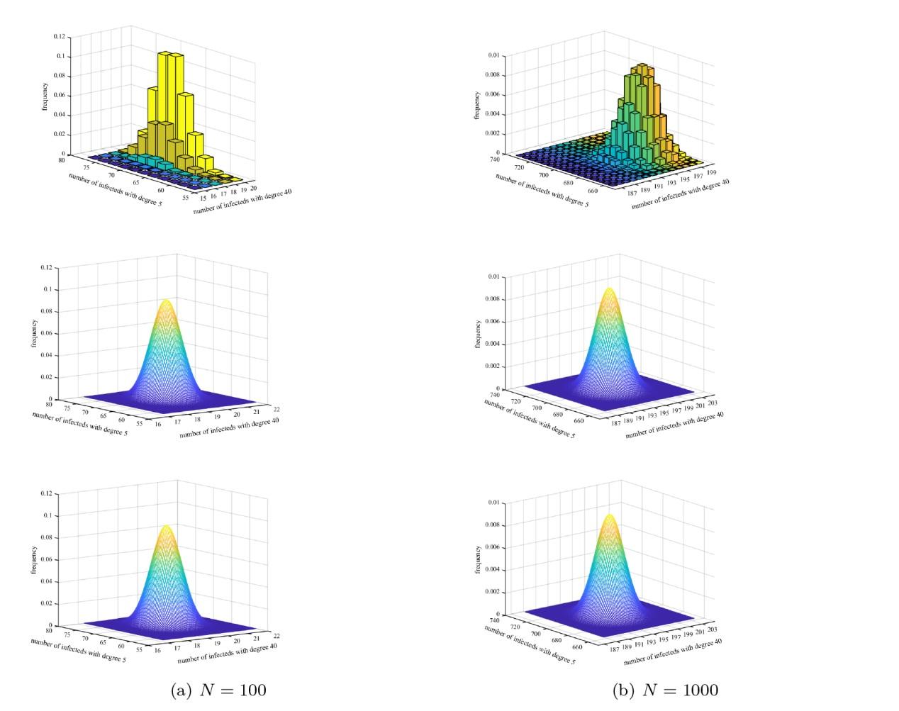
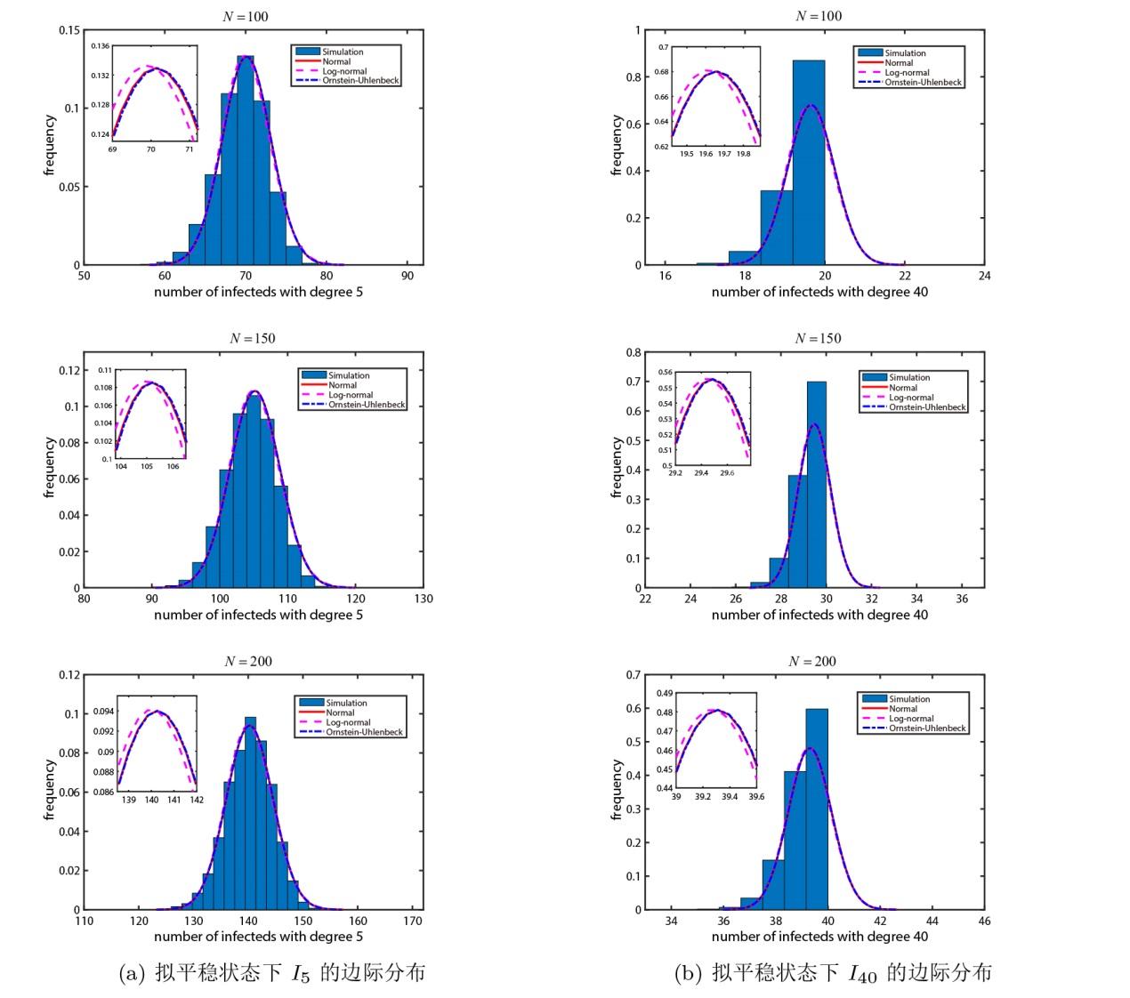
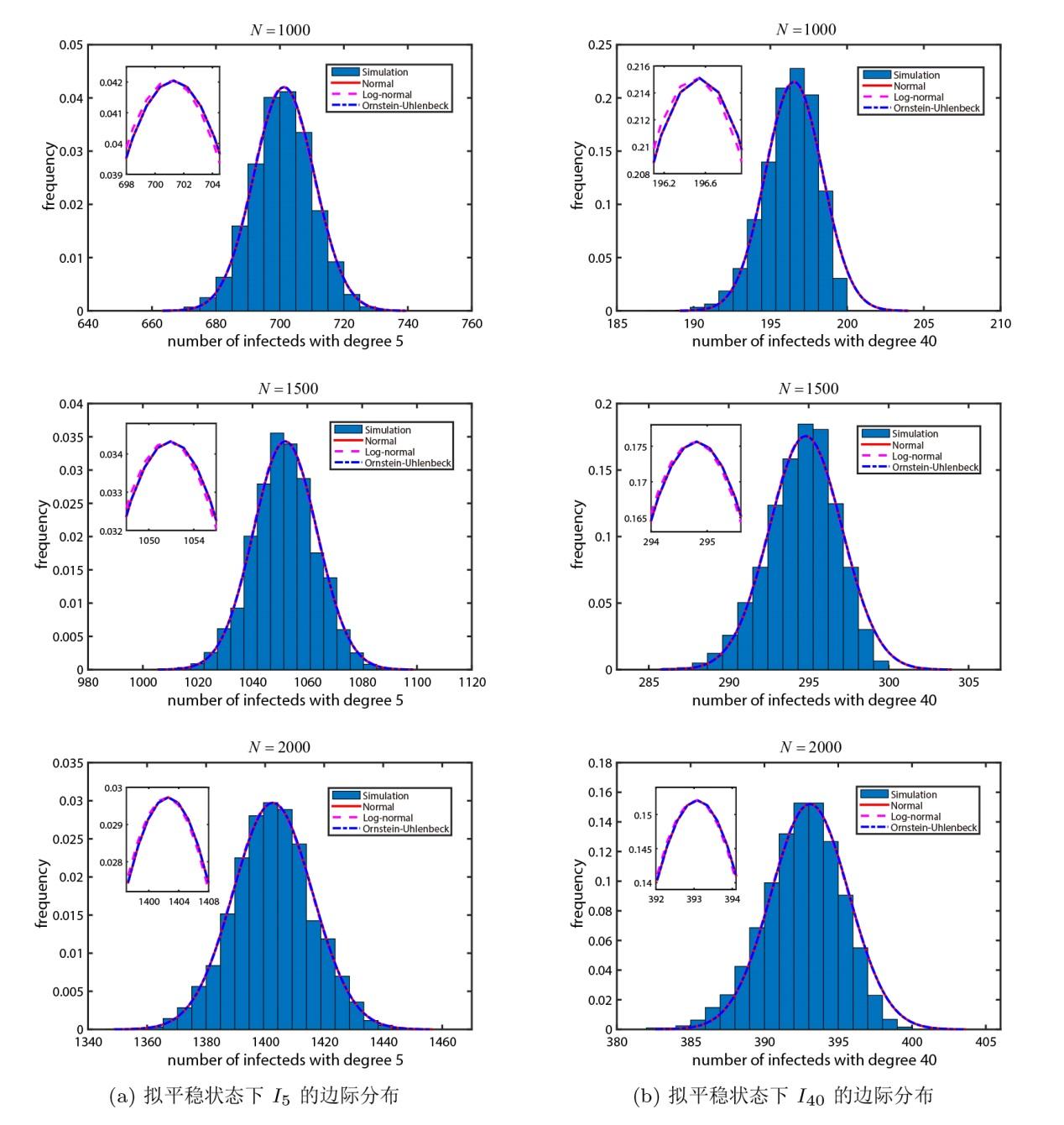
图 1 的最上层为基于蒙特卡洛模拟得到的拟平稳分布 $q_{i_{5},i_{40}}$ 图 2 和图 3 展示拟平稳状态下 $I_{5}$ $I_{40}$
图 1
图 1
种群规模 $N=100$ $N=1000$ $\beta=1.5,~\gamma=1$ .
图 2
图 2
小种群规模下 ($N=100,150,200$ ) 拟平稳分布的近似结果与蒙特卡洛模拟结果.
图 3
图 3
大种群规模下 ($N=1000, 1500, 2000$ ) 拟平稳分布的近似结果与蒙特卡洛模拟结果.
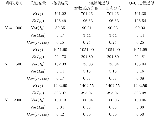
图 2 显示, 在较小种群规模下, 对数正态近似、正态近似和 O-U 过程近似之间存在明显差异. 图 3 表明, 随着种群规模增大, 这三种近似结果趋于一致, 并逐渐接近蒙特卡洛模拟结果. 这一事实在表 2 和表 3 中的定量结果中得到了进一步验证.
表 2 和表 3 展示了不同种群规模下理论计算与蒙特卡洛模拟的结果, 发现当种群规模较小时, 拟平稳分布的对数正态分布近似远优于正态分布近似或 O-U 过程近似. 总体而言, 矩封闭方法能提供比 O-U 过程近似更精确的近似. 这两种方法的结果差异主要体现在均值的近似上. 例如, 从表 2 可以看出, 当 $N=100$ $E(I_{40})\approx19.64$ $E(I_{5})\approx70.09$ $E(I_{40})\approx19.65$ $E(I_{5})\approx70.13$ $E(I_{40})\approx19.64$ $E(I_{5})\approx70.07$ .
4.2 灭绝时间
状态空间 $C$ $\left\{(0,\cdots,0,\cdots,0)\right\}$ $T$ . 记 $Q$ $Q_{T}$ $Q$ $T$ 19 ] 知, 传播过程的拟平稳分布 $\boldsymbol{q}$ $ q_{\boldsymbol{i}}=\lim _{t \rightarrow \infty} \mathrm{P}\{\boldsymbol{I}(t)=\boldsymbol{i} \mid \boldsymbol{I}(t) \in T\},~~i\in T. $ $\boldsymbol{q}$ $ \boldsymbol{q} Q_{\text{d}t}=-\frac{1}{\lambda}\boldsymbol{q},~~\sum_{i\in T}q_{i}=1, $ $-(1/\lambda)$ $Q_{T}$ $\tau_{Q}$ $-(1/\lambda)$
(4.1) $\begin{equation}\label{EQ4.1} E(\tau_{Q})=\lambda. \end{equation}$
图 4 展示了 $\ln\left(E(\tau_{Q})\right)$
图 4
图 4
不同种群规模下 $\ln\left(E(\tau_{Q})\right)$ $\beta=0.5,\,\gamma=5$ .
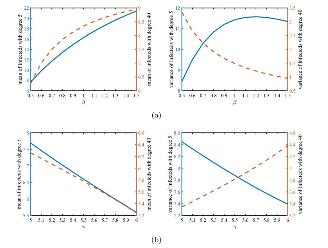
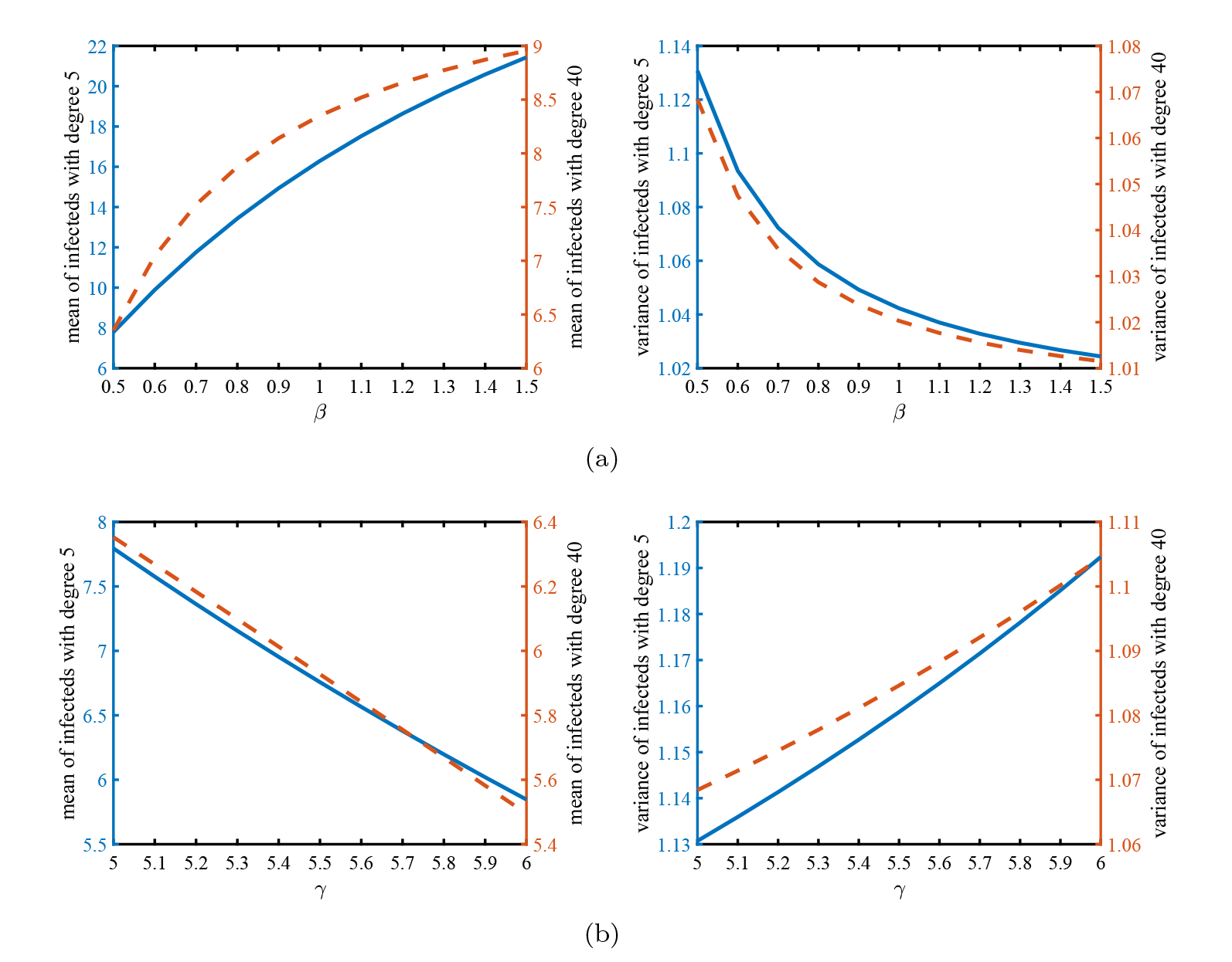
本小节中, 通过数值模拟研究了 $\beta$ $\gamma$ $I_{5}$ $I_{40}$ 图 5 的正态分布近似中可以看出: 对于 $I_{5}$ $\beta$ $\gamma$ $I_{40}$ $\beta$ $\gamma$ $\gamma$ 图 6 的对数正态分布近似中可以看出: $I_{5}$ $I_{40}$ $\beta$ $\gamma$
图 5
图 5
基于正态分布近似, $\beta$ $\gamma$ $I_{5}$ $I_{40}$ $\beta$ $\beta\in[0.5,1.5]$ ) 对拟平稳状态下 $I_{5}$ $I_{40}$ $\gamma=5$ . (b) 展示了 $\gamma$ $\gamma\in$[5 ,6 ] ) 对拟平稳状态下 $I_{5}$ $I_{40}$ $\beta=0.5$ . 人口规模 $N=50$ .
图 6
图 6
基于对数正态分布近似, $\beta$ $\gamma$ $I_{5}$ $I_{40}$ 图 5 相同.
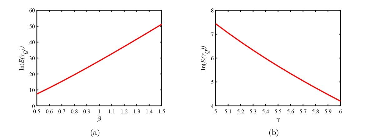
图 7 展示了 $\beta$ $\gamma$ $\ln\left(E(\tau_{Q})\right)$ 图 7(a) 显示了 $\ln\left(E(\tau_{Q})\right)$ $\beta$ $\ln\left(E(\tau_{Q})\right)$ $\beta$ 图 7(b) 显示了 $\ln\left(E(\tau_{Q})\right)$ $\gamma$ $\beta$ $\gamma$ .
图 7
图 7
$\beta$ $\gamma$ $\ln\left(E(\tau_{Q})\right)$ $\beta$ $\beta\in[0.5,1.5]$ ) 对 $\ln\left(E(\tau_{Q})\right)$ $\gamma$ $\gamma\in$[5 ,6 ] ) 对 $\ln\left(E(\tau_{Q})\right)$ $N=50$ .
5 结论
本文关注具有异质群体的随机 SIS 传染病模型的随机动力学, 给出了拟平稳分布的两种近似形式, 正态分布与对数正态分布. 模拟表明对数正态分布的近似效果在不同种群规模下均优于正态分布. 另一个结果是从拟平稳状态开始的平均灭绝时间. 理论分析上, 对数正态分布无法近似平均灭绝时间, 而正态分布在灭绝时间近似上存在显著误差. 对平均灭绝时间的参数敏感性分析表明, 在控制传染病时, 应首先考虑减少传染病暴露的干预措施.
参考文献
View Option
[1]
Dangerfield C E Ross J V Keeling M J Integrating stochasticity and network structure into an epidemic model
J R Soc Interface , 2009 , 6 38 ): 761 -774
DOI:10.1098/rsif.2008.0410
URL
[本文引用: 2]
[2]
Graham M House T Dynamics of stochastic epidemics on heterogeneous networks
J Math Biol , 2014 , 68 7 ): 1583 -1605
DOI:10.1007/s00285-013-0679-1
PMID:23633042
[本文引用: 1]
Epidemic models currently play a central role in our attempts to understand and control infectious diseases. Here, we derive a model for the diffusion limit of stochastic susceptible-infectious-removed (SIR) epidemic dynamics on a heterogeneous network. Using this, we consider analytically the early asymptotic exponential growth phase of such epidemics, showing how the higher order moments of the network degree distribution enter into the stochastic behaviour of the epidemic. We find that the first three moments of the network degree distribution are needed to specify the variance in disease prevalence fully, meaning that the skewness of the degree distribution affects the variance of the prevalence of infection. We compare these asymptotic results to simulation and find a close agreement for city-sized populations.
[3]
Ball F Britton T Leung K Y et al . A stochastic SIR network epidemic model with preventive dropping of edges
J Math Biol , 2019 , 78 6 ): 1875 -1951
DOI:10.1007/s00285-019-01329-4
PMID:30868213
[本文引用: 1]
A Markovian Susceptible [Formula: see text] Infectious [Formula: see text] Recovered (SIR) model is considered for the spread of an epidemic on a configuration model network, in which susceptible individuals may take preventive measures by dropping edges to infectious neighbours. An effective degree formulation of the model is used in conjunction with the theory of density dependent population processes to obtain a law of large numbers and a functional central limit theorem for the epidemic as the population size [Formula: see text], assuming that the degrees of individuals are bounded. A central limit theorem is conjectured for the final size of the epidemic. The results are obtained for both the Molloy-Reed (in which the degrees of individuals are deterministic) and Newman-Strogatz-Watts (in which the degrees of individuals are independent and identically distributed) versions of the configuration model. The two versions yield the same limiting deterministic model but the asymptotic variances in the central limit theorems are greater in the Newman-Strogatz-Watts version. The basic reproduction number [Formula: see text] and the process of susceptible individuals in the limiting deterministic model, for the model with dropping of edges, are the same as for a corresponding SIR model without dropping of edges but an increased recovery rate, though, when [Formula: see text], the probability of a major outbreak is greater in the model with dropping of edges. The results are specialised to the model without dropping of edges to yield conjectured central limit theorems for the final size of Markovian SIR epidemics on configuration-model networks, and for the size of the giant components of those networks. The theory is illustrated by numerical studies, which demonstrate that the asymptotic approximations are good, even for moderate N.
[4]
Achterberg M A Van Mieghem P Moment closure approximations of susceptible-infected-susceptible epidemics on adaptive networks
Phys Rev E , 2022 , 106 1 ): Art 014308
DOI:10.1103/PhysRevE.106.014308
URL
[本文引用: 2]
[5]
Nåsell I An extension of the moment closure method
Theor Popul Biol , 2003 , 64 2 ): 233 -239
PMID:12948684
[本文引用: 4]
The moment closure method was recently shown in Nåsell (Theor. Popul. Biol. 63 (2) (2003a) 159) to give asymptotic approximations of the first few cumulants for the stochastic logistic model. A slight extension of the method is introduced. It is shown to be robust with regard to the specific distributional assumption that is used to achieve moment closure. The phenomenon of spurious solutions is shown to be related to the domain of attraction of the non-spurious critical point.
[6]
Nåsell I Moment closure and the stochastic logistic model
Theor Popul Biol , 2003 , 63 2 ): 159 -168
DOI:10.1016/s0040-5809(02)00060-6
PMID:12615498
[本文引用: 2]
The quasi-stationary distribution of the stochastic logistic model is studied in the parameter region where its body is approximately normal. Improved asymptotic approximations of its first three cumulants are derived. It is shown that the same results can be derived with the aid of the moment closure method. This indicates that the moment closure method leads to expressions for the cumulants that are asymptotic approximations of the cumulants of the quasi-stationary distribution.
[7]
Lloyd A L Estimating variability in models for recurrent epidemics: assessing the use of moment closure techniques
Theor Popul Biol , 2004 , 65 1 ): 49 -65
PMID:14642344
The major role played by demographic stochasticity in determining the dynamics and persistence of childhood diseases, such as measles, chickenpox and pertussis, has long been realized. Techniques which can be used to estimate the magnitude of this stochastic effect are of clear importance. In this study, we assess and compare the use of two moment closure approximations to estimate the variability seen about the average behavior of stochastic models for the recurrent epidemics seen in childhood diseases. The performance of the approximations are assessed using analytic techniques available for the simplest epidemiological model and using numerical simulations in more complex settings. We also present epidemiologically important extensions of previous work, considering variability in the SEIR model and in situations for which there is seasonal variation in disease transmission. Important implications of stochastic effects for the dynamics of childhood diseases are highlighted, including serious deficiencies of deterministic descriptions of dynamical behavior.
[8]
Clancy D Mendy S T The effect of waning immunity on long-term behaviour of stochastic models for the spread of infection
J Math Biol , 2010 , 61 4 ): 527 -544
DOI:10.1007/s00285-009-0313-4
PMID:19941137
In stochastic modelling of infectious spread, it is often assumed that infection confers permanent immunity, a susceptible-infective-removed (SIR) model. We show how results concerning long-term (endemic) behaviour may be extended to a susceptible-infective-removed-susceptible (SIRS) model, in which immunity is temporary. Since the full SIRS model with demography is rather intractable, we also consider two simpler models: the susceptible-infective-susceptible (SIS) model with demography, in which there is no immunity; and the SIRS model in a closed population. For each model, we first analyse a deterministic model, then approximate the quasi-stationary distribution (equilibrium distribution conditional upon non-extinction of infection) using a moment closure technique. We look in particular at the effect of the immune period upon infection prevalence and upon time to fade-out of infection. Our main findings are that a shorter average immune period leads to higher infection prevalence in quasi-stationarity, and to longer persistence of infection in the population.
[9]
Clancy D Mendy S T Approximating the quasi-stationary distribution of the SIS model for endemic infection
Methodol Comput Appl , 2011 , 13 3 ): 603 -618
[本文引用: 1]
[10]
Isham V Assessing the variability of stochastic epidemics
Math Biosci , 1991 , 107 2 ): 207 -224
[本文引用: 1]
[12]
Allen, L J S An Introduction to Stochastic Processes with Applications to Biology . Florida : CRC Press , 2010
[本文引用: 1]
[13]
Pastor-Satorras R Vespignani A Epidemic spreading in scale-free networks
Phys Rev Lett , 2001 , 86 14 ): 3200 -3203
PMID:11290142
[本文引用: 1]
The Internet has a very complex connectivity recently modeled by the class of scale-free networks. This feature, which appears to be very efficient for a communications network, favors at the same time the spreading of computer viruses. We analyze real data from computer virus infections and find the average lifetime and persistence of viral strains on the Internet. We define a dynamical model for the spreading of infections on scale-free networks, finding the absence of an epidemic threshold and its associated critical behavior. This new epidemiological framework rationalizes data of computer viruses and could help in the understanding of other spreading phenomena on communication and social networks.
[16]
Keeling M J Metapopulation moments: coupling, stochasticity and persistence
J Anim Ecol , 2000 , 69 5 ): 725 -736
DOI:10.1046/j.1365-2656.2000.00430.x
PMID:29314000
[本文引用: 1]
1. Spatial heterogeneity has long been viewed as a reliable means of increasing persistence. Here, an analytical model is developed to consider the variation and, hence, the persistence of stochastic metapopulations. This model relies on a novel moment closure technique, which is equivalent to assuming log-normal distributions for the population sizes. 2. Single-species models show the greatest persistence when the mixing between subpopulations is large, so spatial heterogeneity is of no benefit. This result is confirmed by stochastic simulation of the full metapopulation. 3. In contrast, natural-enemy models exhibit the greatest persistence for intermediate levels of coupling. When the coupling is too low, there are insufficient rescue effects between the subpopulations to sustain the dynamics, whereas when the coupling is too high all spatial heterogeneity is lost. 4. The difference in behaviour between the one- and two-species models can be attributed to the oscillatory nature of the natural-enemy system.
[17]
Keeling M J Multiplicative moments and measures of persistence in ecology
J Theor Biol , 2000 , 205 2 ): 269 -281
PMID:10873438
[本文引用: 1]
Ecologists and epidemiologists have begun focusing on demographic stochasticity and spatial heterogeneity as important biological factors. With high-powered computers simulation of such systems is a common modelling technique; however we lack a detailed understanding of the processes involved. Moment closure approximations provide a simple method which can be used to capture the main features of a wide variety of stochastic models and to gain a more intuitive understanding. In this paper we give an alternative variation based on multiplicative moments which is equivalent to taking a novel third-order cumulant approximation. The differential equations for these multiplicative moments are far more robust than their additive counterparts. We use this technique to consider the behaviour and persistence of finite metapopulations for two common ecological systems.Copyright 2000 Academic Press.
[18]
Britton T Traoré A A stochastic vector-borne epidemic model: Quasi-stationarity and extinction
Math Biosci , 2017 , 289 89 -95
DOI:S0025-5564(17)30268-7
PMID:28511957
[本文引用: 1]
We consider a stochastic model describing the spread of a vector borne disease in a community where individuals (hosts and vectors) die and new individuals (hosts and vectors) are born. The time to extinction of the disease, T, starting in quasi-stationary (conditional on non extinction) is studied. Properties of the limiting distribution are used to obtain an approximate expression for E(T), the mean-parameter in the exponential distribution of the time to extinction, for a finite population. It is then investigated numerically and by means of simulations how E(T) and its approximations depend on the different model parameters.Copyright © 2017 Elsevier Inc. All rights reserved.
[19]
Darroch J N Seneta E On quasi-stationary distributions in absorbing continuous-time finite Markov chains
J Appl Probab , 1967 , 4 1 ): 192 -196
DOI:10.2307/3212311
URL
[本文引用: 1]
Integrating stochasticity and network structure into an epidemic model
2
2009
... 近年来, 基于网络传染病模型的随机动力学研究受到关注 [1 4 ] . Dangerfield 等 [1 ] 利用扩散近似, 研究了空间结构和随机性在 SIS 型传染病传播中的影响. Graham 和 House[2 ] 探究了异质网络上 SIR 型传染病在早期指数增长阶段的渐近方差. Ball 等 [3 ] 给出了异质网络上 SIR 型传染病的最终规模. Achterberg 和 Van Mieghem[4 ] 推导了广义自适应网络上马尔可夫 SIS 模型的平均场近似. 然而, 关于一般异质网络上传播过程的拟平稳分布的研究仍为有限. ...
... [1 ]利用扩散近似, 研究了空间结构和随机性在 SIS 型传染病传播中的影响. Graham 和 House[2 ] 探究了异质网络上 SIR 型传染病在早期指数增长阶段的渐近方差. Ball 等 [3 ] 给出了异质网络上 SIR 型传染病的最终规模. Achterberg 和 Van Mieghem[4 ] 推导了广义自适应网络上马尔可夫 SIS 模型的平均场近似. 然而, 关于一般异质网络上传播过程的拟平稳分布的研究仍为有限. ...
Dynamics of stochastic epidemics on heterogeneous networks
1
2014
... 近年来, 基于网络传染病模型的随机动力学研究受到关注 [1 4 ] . Dangerfield 等 [1 ] 利用扩散近似, 研究了空间结构和随机性在 SIS 型传染病传播中的影响. Graham 和 House[2 ] 探究了异质网络上 SIR 型传染病在早期指数增长阶段的渐近方差. Ball 等 [3 ] 给出了异质网络上 SIR 型传染病的最终规模. Achterberg 和 Van Mieghem[4 ] 推导了广义自适应网络上马尔可夫 SIS 模型的平均场近似. 然而, 关于一般异质网络上传播过程的拟平稳分布的研究仍为有限. ...
A stochastic SIR network epidemic model with preventive dropping of edges
1
2019
... 近年来, 基于网络传染病模型的随机动力学研究受到关注 [1 4 ] . Dangerfield 等 [1 ] 利用扩散近似, 研究了空间结构和随机性在 SIS 型传染病传播中的影响. Graham 和 House[2 ] 探究了异质网络上 SIR 型传染病在早期指数增长阶段的渐近方差. Ball 等 [3 ] 给出了异质网络上 SIR 型传染病的最终规模. Achterberg 和 Van Mieghem[4 ] 推导了广义自适应网络上马尔可夫 SIS 模型的平均场近似. 然而, 关于一般异质网络上传播过程的拟平稳分布的研究仍为有限. ...
Moment closure approximations of susceptible-infected-susceptible epidemics on adaptive networks
2
2022
... 近年来, 基于网络传染病模型的随机动力学研究受到关注 [1 4 ] . Dangerfield 等 [1 ] 利用扩散近似, 研究了空间结构和随机性在 SIS 型传染病传播中的影响. Graham 和 House[2 ] 探究了异质网络上 SIR 型传染病在早期指数增长阶段的渐近方差. Ball 等 [3 ] 给出了异质网络上 SIR 型传染病的最终规模. Achterberg 和 Van Mieghem[4 ] 推导了广义自适应网络上马尔可夫 SIS 模型的平均场近似. 然而, 关于一般异质网络上传播过程的拟平稳分布的研究仍为有限. ...
... [4 ] 推导了广义自适应网络上马尔可夫 SIS 模型的平均场近似. 然而, 关于一般异质网络上传播过程的拟平稳分布的研究仍为有限. ...
An extension of the moment closure method
4
2003
... 研究拟平稳分布常用的方法之一是矩封闭近似 [5 9 ] , 即通过系统状态分布的矩来研究传染病传播中的变异性[10 ,11 ] . 一般而言, 矩方程是无限维的, 无法直接处理. 因此, 需要给定分布, 利用该分布矩之间的关系对方程组进行截断, 以获得低阶矩方程. 现有研究在均匀混合层面上评估了给定分布在矩封闭方法上的近似效果, 忽略了传播过程中个体异质性. 本文将该方法推广到异质网络上, 假设传播过程处于阈值之上 (即 $R_{0}>1$ ) , 研究传染病的随机动力学行为. ...
... 根据文献[13 ,14 ], 可知 $R_{0}=\beta(\sigma^{2}_{D}+\mu^{2}_{D})/(\gamma\mu_{D})$ $\sigma^{2}_{D}$ 5 ,15 ], 当 $R_{0}>1$ $q_{e_{l}}\,(l=1,\cdots,K)$ $q_{e_{l}}(t)\,(l=1,\cdots,K)$
... 本小节中, 通过数值模拟研究了
$\beta$ 和
$\gamma$ 对拟平稳状态下
$I_{5}$ 和
$I_{40}$ 的均值与方差的影响. 从
图 5 的正态分布近似中可以看出: 对于
$I_{5}$ , 均值随
$\beta$ 增大而增大, 方差则先增大后减小; 均值和方差均随
$\gamma$ 增大而减小. 对于
$I_{40}$ , 均值随
$\beta$ 增大而增大, 而方差随之减小; 均值随
$\gamma$ 增大而减小, 方差随
$\gamma$ 增大而增大. 从
图 6 的对数正态分布近似中可以看出:
$I_{5}$ 和
$I_{40}$ 的均值均随
$\beta$ 增大而增大, 但方差随之增大而减小; 两者均值随
$\gamma$ 增大而减小, 方差随之增大而增大.
图 5 基于正态分布近似, <span class="formulaText"><inline-formula>$\beta$</inline-formula></span> 和 <span class="formulaText"><inline-formula>$\gamma$</inline-formula></span> 对拟平稳状态下 <span class="formulaText"><inline-formula>$I_{5}$</inline-formula></span> 和 <span class="formulaText"><inline-formula>$I_{40}$</inline-formula></span> 的均值与方差的影响. (a) 展示了 <span class="formulaText"><inline-formula>$\beta$</inline-formula></span> (<span class="formulaText"><inline-formula>$\beta\in[0.5,1.5]$</inline-formula></span><span class="formulaNumber">)</span> 对拟平稳状态下 <span class="formulaText"><inline-formula>$I_{5}$</inline-formula></span> 和 <span class="formulaText"><inline-formula>$I_{40}$</inline-formula></span> 的均值与方差的影响, 其中 <span class="formulaText"><inline-formula>$\gamma=5$</inline-formula></span><span class="formulaNumber">.</span> (b) 展示了 <span class="formulaText"><inline-formula>$\gamma$</inline-formula></span> (<span class="formulaText"><inline-formula>$\gamma\in$<sup>[<xref ref-type="bibr" rid="b5">5</xref>,<xref ref-type="bibr" rid="b6">6</xref>]</sup></inline-formula></span><span class="formulaNumber">)</span> 对拟平稳状态下 <span class="formulaText"><inline-formula>$I_{5}$</inline-formula></span> 和 <span class="formulaText"><inline-formula>$I_{40}$</inline-formula></span> 的均值与方差的影响, 其中 <span class="formulaText"><inline-formula>$\beta=0.5$</inline-formula></span><span class="formulaNumber">.</span> 人口规模 <span class="formulaText"><inline-formula>$N=50$</inline-formula></span><span class="formulaNumber">.</span> ![]()
图 6 基于对数正态分布近似, <span class="formulaText"><inline-formula>$\beta$</inline-formula></span> 和 <span class="formulaText"><inline-formula>$\gamma$</inline-formula></span> 对拟平稳状态下 <span class="formulaText"><inline-formula>$I_{5}$</inline-formula></span> 和 <span class="formulaText"><inline-formula>$I_{40}$</inline-formula></span> 的均值与方差的影响. (a) 和 (b) 的参数设置与<xref ref-type="fig" rid="F5">图 5</xref> 相同. ![]()
图 7 展示了 $\beta$ $\gamma$ $\ln\left(E(\tau_{Q})\right)$ 图 7(a) 显示了 $\ln\left(E(\tau_{Q})\right)$ $\beta$ $\ln\left(E(\tau_{Q})\right)$ $\beta$ 图 7(b) 显示了 $\ln\left(E(\tau_{Q})\right)$ $\gamma$ $\beta$ $\gamma$ . ...
...
图 7 展示了
$\beta$ 和
$\gamma$ 对
$\ln\left(E(\tau_{Q})\right)$ 的影响.
图 7(a) 显示了
$\ln\left(E(\tau_{Q})\right)$ 和
$\beta$ 的线性关系, 且
$\ln\left(E(\tau_{Q})\right)$ 随
$\beta$ 的增大而单调递增. 类似地,
图 7(b) 显示了
$\ln\left(E(\tau_{Q})\right)$ 随
$\gamma$ 的增大而线性减小. 此外可以看出, 影响最大的参数是
$\beta$ , 其次是
$\gamma$ . 图 7 <span class="formulaText"><inline-formula>$\beta$</inline-formula></span> 和 <span class="formulaText"><inline-formula>$\gamma$</inline-formula></span> 对 <span class="formulaText"><inline-formula>$\ln\left(E(\tau_{Q})\right)$</inline-formula></span> 的影响. (a) 展示了 <span class="formulaText"><inline-formula>$\beta$</inline-formula></span> (<span class="formulaText"><inline-formula>$\beta\in[0.5,1.5]$</inline-formula></span><span class="formulaNumber">)</span> 对 <span class="formulaText"><inline-formula>$\ln\left(E(\tau_{Q})\right)$</inline-formula></span> 的影响. (b) 展示了 <span class="formulaText"><inline-formula>$\gamma$</inline-formula></span> (<span class="formulaText"><inline-formula>$\gamma\in$<sup>[<xref ref-type="bibr" rid="b5">5</xref>,<xref ref-type="bibr" rid="b6">6</xref>]</sup></inline-formula></span><span class="formulaNumber">)</span> 对 <span class="formulaText"><inline-formula>$\ln\left(E(\tau_{Q})\right)$</inline-formula></span> 的影响. 人口规模 <span class="formulaText"><inline-formula>$N=50$</inline-formula></span><span class="formulaNumber">.</span> ![]()
5 结论 本文关注具有异质群体的随机 SIS 传染病模型的随机动力学, 给出了拟平稳分布的两种近似形式, 正态分布与对数正态分布. 模拟表明对数正态分布的近似效果在不同种群规模下均优于正态分布. 另一个结果是从拟平稳状态开始的平均灭绝时间. 理论分析上, 对数正态分布无法近似平均灭绝时间, 而正态分布在灭绝时间近似上存在显著误差. 对平均灭绝时间的参数敏感性分析表明, 在控制传染病时, 应首先考虑减少传染病暴露的干预措施. ...
Moment closure and the stochastic logistic model
2
2003
... 本小节中, 通过数值模拟研究了
$\beta$ 和
$\gamma$ 对拟平稳状态下
$I_{5}$ 和
$I_{40}$ 的均值与方差的影响. 从
图 5 的正态分布近似中可以看出: 对于
$I_{5}$ , 均值随
$\beta$ 增大而增大, 方差则先增大后减小; 均值和方差均随
$\gamma$ 增大而减小. 对于
$I_{40}$ , 均值随
$\beta$ 增大而增大, 而方差随之减小; 均值随
$\gamma$ 增大而减小, 方差随
$\gamma$ 增大而增大. 从
图 6 的对数正态分布近似中可以看出:
$I_{5}$ 和
$I_{40}$ 的均值均随
$\beta$ 增大而增大, 但方差随之增大而减小; 两者均值随
$\gamma$ 增大而减小, 方差随之增大而增大.
图 5 基于正态分布近似, <span class="formulaText"><inline-formula>$\beta$</inline-formula></span> 和 <span class="formulaText"><inline-formula>$\gamma$</inline-formula></span> 对拟平稳状态下 <span class="formulaText"><inline-formula>$I_{5}$</inline-formula></span> 和 <span class="formulaText"><inline-formula>$I_{40}$</inline-formula></span> 的均值与方差的影响. (a) 展示了 <span class="formulaText"><inline-formula>$\beta$</inline-formula></span> (<span class="formulaText"><inline-formula>$\beta\in[0.5,1.5]$</inline-formula></span><span class="formulaNumber">)</span> 对拟平稳状态下 <span class="formulaText"><inline-formula>$I_{5}$</inline-formula></span> 和 <span class="formulaText"><inline-formula>$I_{40}$</inline-formula></span> 的均值与方差的影响, 其中 <span class="formulaText"><inline-formula>$\gamma=5$</inline-formula></span><span class="formulaNumber">.</span> (b) 展示了 <span class="formulaText"><inline-formula>$\gamma$</inline-formula></span> (<span class="formulaText"><inline-formula>$\gamma\in$<sup>[<xref ref-type="bibr" rid="b5">5</xref>,<xref ref-type="bibr" rid="b6">6</xref>]</sup></inline-formula></span><span class="formulaNumber">)</span> 对拟平稳状态下 <span class="formulaText"><inline-formula>$I_{5}$</inline-formula></span> 和 <span class="formulaText"><inline-formula>$I_{40}$</inline-formula></span> 的均值与方差的影响, 其中 <span class="formulaText"><inline-formula>$\beta=0.5$</inline-formula></span><span class="formulaNumber">.</span> 人口规模 <span class="formulaText"><inline-formula>$N=50$</inline-formula></span><span class="formulaNumber">.</span> ![]()
图 6 基于对数正态分布近似, <span class="formulaText"><inline-formula>$\beta$</inline-formula></span> 和 <span class="formulaText"><inline-formula>$\gamma$</inline-formula></span> 对拟平稳状态下 <span class="formulaText"><inline-formula>$I_{5}$</inline-formula></span> 和 <span class="formulaText"><inline-formula>$I_{40}$</inline-formula></span> 的均值与方差的影响. (a) 和 (b) 的参数设置与<xref ref-type="fig" rid="F5">图 5</xref> 相同. ![]()
图 7 展示了 $\beta$ $\gamma$ $\ln\left(E(\tau_{Q})\right)$ 图 7(a) 显示了 $\ln\left(E(\tau_{Q})\right)$ $\beta$ $\ln\left(E(\tau_{Q})\right)$ $\beta$ 图 7(b) 显示了 $\ln\left(E(\tau_{Q})\right)$ $\gamma$ $\beta$ $\gamma$ . ...
...
图 7 展示了
$\beta$ 和
$\gamma$ 对
$\ln\left(E(\tau_{Q})\right)$ 的影响.
图 7(a) 显示了
$\ln\left(E(\tau_{Q})\right)$ 和
$\beta$ 的线性关系, 且
$\ln\left(E(\tau_{Q})\right)$ 随
$\beta$ 的增大而单调递增. 类似地,
图 7(b) 显示了
$\ln\left(E(\tau_{Q})\right)$ 随
$\gamma$ 的增大而线性减小. 此外可以看出, 影响最大的参数是
$\beta$ , 其次是
$\gamma$ . 图 7 <span class="formulaText"><inline-formula>$\beta$</inline-formula></span> 和 <span class="formulaText"><inline-formula>$\gamma$</inline-formula></span> 对 <span class="formulaText"><inline-formula>$\ln\left(E(\tau_{Q})\right)$</inline-formula></span> 的影响. (a) 展示了 <span class="formulaText"><inline-formula>$\beta$</inline-formula></span> (<span class="formulaText"><inline-formula>$\beta\in[0.5,1.5]$</inline-formula></span><span class="formulaNumber">)</span> 对 <span class="formulaText"><inline-formula>$\ln\left(E(\tau_{Q})\right)$</inline-formula></span> 的影响. (b) 展示了 <span class="formulaText"><inline-formula>$\gamma$</inline-formula></span> (<span class="formulaText"><inline-formula>$\gamma\in$<sup>[<xref ref-type="bibr" rid="b5">5</xref>,<xref ref-type="bibr" rid="b6">6</xref>]</sup></inline-formula></span><span class="formulaNumber">)</span> 对 <span class="formulaText"><inline-formula>$\ln\left(E(\tau_{Q})\right)$</inline-formula></span> 的影响. 人口规模 <span class="formulaText"><inline-formula>$N=50$</inline-formula></span><span class="formulaNumber">.</span> ![]()
5 结论 本文关注具有异质群体的随机 SIS 传染病模型的随机动力学, 给出了拟平稳分布的两种近似形式, 正态分布与对数正态分布. 模拟表明对数正态分布的近似效果在不同种群规模下均优于正态分布. 另一个结果是从拟平稳状态开始的平均灭绝时间. 理论分析上, 对数正态分布无法近似平均灭绝时间, 而正态分布在灭绝时间近似上存在显著误差. 对平均灭绝时间的参数敏感性分析表明, 在控制传染病时, 应首先考虑减少传染病暴露的干预措施. ...
Estimating variability in models for recurrent epidemics: assessing the use of moment closure techniques
0
2004
The effect of waning immunity on long-term behaviour of stochastic models for the spread of infection
0
2010
Approximating the quasi-stationary distribution of the SIS model for endemic infection
1
2011
... 研究拟平稳分布常用的方法之一是矩封闭近似 [5 9 ] , 即通过系统状态分布的矩来研究传染病传播中的变异性[10 ,11 ] . 一般而言, 矩方程是无限维的, 无法直接处理. 因此, 需要给定分布, 利用该分布矩之间的关系对方程组进行截断, 以获得低阶矩方程. 现有研究在均匀混合层面上评估了给定分布在矩封闭方法上的近似效果, 忽略了传播过程中个体异质性. 本文将该方法推广到异质网络上, 假设传播过程处于阈值之上 (即 $R_{0}>1$ ) , 研究传染病的随机动力学行为. ...
Assessing the variability of stochastic epidemics
1
1991
... 研究拟平稳分布常用的方法之一是矩封闭近似 [5 9 ] , 即通过系统状态分布的矩来研究传染病传播中的变异性[10 ,11 ] . 一般而言, 矩方程是无限维的, 无法直接处理. 因此, 需要给定分布, 利用该分布矩之间的关系对方程组进行截断, 以获得低阶矩方程. 现有研究在均匀混合层面上评估了给定分布在矩封闭方法上的近似效果, 忽略了传播过程中个体异质性. 本文将该方法推广到异质网络上, 假设传播过程处于阈值之上 (即 $R_{0}>1$ ) , 研究传染病的随机动力学行为. ...
On the use of the normal approximation in the treatment of stochastic processes
1
1957
... 研究拟平稳分布常用的方法之一是矩封闭近似 [5 9 ] , 即通过系统状态分布的矩来研究传染病传播中的变异性[10 ,11 ] . 一般而言, 矩方程是无限维的, 无法直接处理. 因此, 需要给定分布, 利用该分布矩之间的关系对方程组进行截断, 以获得低阶矩方程. 现有研究在均匀混合层面上评估了给定分布在矩封闭方法上的近似效果, 忽略了传播过程中个体异质性. 本文将该方法推广到异质网络上, 假设传播过程处于阈值之上 (即 $R_{0}>1$ ) , 研究传染病的随机动力学行为. ...
1
2010
... 根据文献[12 ], 前向 Kolmogorov 微分方程如下 ...
Epidemic spreading in scale-free networks
1
2001
... 根据文献[13 ,14 ], 可知 $R_{0}=\beta(\sigma^{2}_{D}+\mu^{2}_{D})/(\gamma\mu_{D})$ $\sigma^{2}_{D}$ 5 ,15 ], 当 $R_{0}>1$ $q_{e_{l}}\,(l=1,\cdots,K)$ $q_{e_{l}}(t)\,(l=1,\cdots,K)$
Epidemic dynamics in finite size scale-free networks
1
2002
... 根据文献[13 ,14 ], 可知 $R_{0}=\beta(\sigma^{2}_{D}+\mu^{2}_{D})/(\gamma\mu_{D})$ $\sigma^{2}_{D}$ 5 ,15 ], 当 $R_{0}>1$ $q_{e_{l}}\,(l=1,\cdots,K)$ $q_{e_{l}}(t)\,(l=1,\cdots,K)$
An alternative to moment closure
1
2017
... 根据文献[13 ,14 ], 可知 $R_{0}=\beta(\sigma^{2}_{D}+\mu^{2}_{D})/(\gamma\mu_{D})$ $\sigma^{2}_{D}$ 5 ,15 ], 当 $R_{0}>1$ $q_{e_{l}}\,(l=1,\cdots,K)$ $q_{e_{l}}(t)\,(l=1,\cdots,K)$
Metapopulation moments: coupling, stochasticity and persistence
1
2000
... $l,m,n=1,\cdots,K$ . 使用文献[16 ,17 ], $\hat{T}_{I_{l}I_{m}I_{n}}=\hat{T}_{I_{l}I_{m}^{2}}=1,\,l,m,n=1,\cdots,K$
Multiplicative moments and measures of persistence in ecology
1
2000
... $l,m,n=1,\cdots,K$ . 使用文献[16 ,17 ], $\hat{T}_{I_{l}I_{m}I_{n}}=\hat{T}_{I_{l}I_{m}^{2}}=1,\,l,m,n=1,\cdots,K$
A stochastic vector-borne epidemic model: Quasi-stationarity and extinction
1
2017
... 证 根据文献[18 ], $\tau_{Q}$ $\gamma\sum_{k=1}^{K}q_{e_{k}}$ . 因此, $E(\tau_{Q})$
On quasi-stationary distributions in absorbing continuous-time finite Markov chains
1
1967
... 状态空间 $C$ $\left\{(0,\cdots,0,\cdots,0)\right\}$ $T$ . 记 $Q$ $Q_{T}$ $Q$ $T$ 19 ] 知, 传播过程的拟平稳分布 $\boldsymbol{q}$ $ q_{\boldsymbol{i}}=\lim _{t \rightarrow \infty} \mathrm{P}\{\boldsymbol{I}(t)=\boldsymbol{i} \mid \boldsymbol{I}(t) \in T\},~~i\in T. $ $\boldsymbol{q}$ $ \boldsymbol{q} Q_{\text{d}t}=-\frac{1}{\lambda}\boldsymbol{q},~~\sum_{i\in T}q_{i}=1, $ $-(1/\lambda)$ $Q_{T}$ $\tau_{Q}$ $-(1/\lambda)$