1 引言
排序集抽样 (Ranked set sampling, RSS )是一种试图用来提高抽样效率的方法, 由澳大利亚农业学家 McIntyre[1 ] 在估计农场牧草产量均值时提出, 近年来已得到了广泛的研究和应用, 见文献[2 6]. RSS 适用于那些对所研究的变量进行精确测量既困难又耗时漫长, 但是在一个相对小的集合中可以通过非精确测量手段进行排序的场合.
(1 )从总体中随机抽取集合大小为 $m$ $n$
(2 )对每个集合中的个体进行不涉及具体测量的排序;
(3 )从排好次序的每个集合中选取一个个体进行测量. 令 ${r_i}$ $i$ $\sum\limits_{i = 1}^m {{r_i}}$ $i = 1,2, \cdots,m$ . 当 ${r_i}$
Takahasi 和 Wakimoto[7 ] 建立了 RSS 的数学理论基础, 并证明了平衡 RSS 下用样本均值作为总体均值的估计比简单随机抽样 (Simple Ranked Set Sampling, SRS )用样本均值作为总体均值的估计更有效.
因为排序不经过测量, 所以合理选择 RSS 的集合大小 $m$ [8 ] 指出集合大小 $m$
平衡 RSS 适用于总体分布完全未知时的统计推断, 但如果已有总体分布的某些信息时, 使用某些准则就可以进一步提高统计推断的效率, 见文献[9 13].
Al-Saleh[14 ] 在均方误差 (MSE )最小准则下, 针对正态分布、均匀分布和指数分布找到了总体均值估计的 3×3 最优 RSS 设计.
本文在文献[14 ] 的基础上, 基于 MSE 最小准则下, 针对正态分布、均匀分布和指数分布找到了总体均值估计的 4×4 最优 RSS 设计. 为了进一步提高估计的精度, 本文研究了这些分布在可循环 4×4 最优 RSS 设计下总体均值估计的 MSE, 研究结果表明在可循环 4×4 最优 RSS 设计下这些分布中总体均值估计的 MSE 随着循环的增大不断减小.
本文的结构安排如下: 第 2 节给出了 4×4 RSS 设计下总体均值估计的 MSE 及其 35 种设计; 第 3 节给出了可循环 4×4 最优 RSS 设计下总体均值的估计及其 MSE; 第 4 节计算了基于 MSE 最小准则下正态分布、均匀分布和指数分布中总体均值估计的 4×4 最优 RSS 设计; 第 5 节计算了可循环 4×4 最优 RSS 设计下这些分布中总体均值估计的 MSE; 第 6 节给出了本文的结语.
2 4×4 RSS 设计下总体均值估计的 MSE 及其 35 种设计
本节从理论上给出了 4×4 RSS 设计下总体均值估计的 MSE, 并列出了 4×4 RSS 设计下的 35 种设计.
2.1 4×4 RSS 设计下总体均值估计的 MSE
(1)从总体中随机抽取集合大小为 4 个个体的 4 个集合;
(2)对每个集合中的个体进行不涉及具体测量的排序;
(3)从排好次序的 4 个集合中分别选取一个个体进行测量. 令 ${r_i}$ $i$ $4 = \sum\limits_{i = 1}^4 {{r_i}}$ ${{\rm{r}}_i}{\rm{ = 0, 1, 2, 3, 4,i = 1, 2, 3, 4}}$ . 当 ${r_i}$
设随机变量 $X$ $F(x)$ $f(x)$ $\mu $ ${\sigma ^2}$ . 令 $\left\{ {\bigcup\limits_{j = 1}^{{r_1}} {{X_{(1:4)j}}} \bigcup\limits_{j = 1}^{{r_2}} {{X_{(2:4)j}}} \bigcup\limits_{j = 1}^{{r_3}} {{X_{(3:4)j}}} \bigcup\limits_{j = 1}^{{r_4}} {{X_{(4:4)j}}} } \right\}$ $X$ ${X_{(i:4)j}}$ $i$ $j$ $({r_1},{r_2},{r_3},{r_4}) = (2,2,0,0)$ $r_{3}=r_{4}=0$ .
令 ${\mu _{(i:m)}}$ $\sigma _{(i:m)}^2$ $i$ ${X_{(1:4)j}},{X_{(2:4)j}},{X_{(3:4)j}}$ ${X_{(4:4)j}}$
(2.1) $\begin{equation} {f_{(1:4)}}(x) = 4{\left[ {1 - F(x)} \right]^3}f(x), \end{equation}$
(2.2) $\begin{equation} {f_{(2:4)}}(x) = 12\left[ {F(x)} \right]{\left[ {1 - F(x)} \right]^2}f(x), \end{equation}$
(2.3) $\begin{equation} {f_{(3:4)}}(x) = 12{\left[ {F(x)} \right]^2}\left[ {1 - F(x)} \right]f(x) \end{equation}$
(2.4) $\begin{equation} {f_{(4:4)}}(x) = 4{\left[ {F(x)} \right]^3}f(x). \end{equation}$
接着, 我们给出 ${\bar X_{RSS}}$
定理 2.1 对于 4×4 RSS 样本, ${\bar X_{RSS}}$
(2.5) $\begin{equation} \begin{aligned} \mathrm{MSE}{({{\bar X}_{RSS}})^{({r_1},{r_2},{r_3},{r_4})}} &= \frac{1}{{16}}({r_1}\sigma _{(1:4)}^2 + {r_2}\sigma _{(2:4)}^2 + {r_3}\sigma _{(3:4)}^2 + {r_4}\sigma _{(4:4)}^2)\\ & + {\left[ {\frac{1}{4}({r_1}{\mu _{(1:4)}} + {r_2}{\mu _{(2:4)}} + {r_3}{\mu _{(3:4)}} + {r_4}{\mu _{(4:4)}}) - \mu } \right]^2}. \end{aligned} \end{equation}$
证 ${\bar X_{RSS}}$
注意, 定理 2.1 表明 ${\bar X_{RSS}}$ ${r_i}$ ${\mu _{(i:4)}}$ $\sigma _{(i:4)}^2$ . 这个特性具有重要的使用价值, 将在本文第 4 节和第 5 节中得到充分体现.
2.2 35 种 RSS 设计
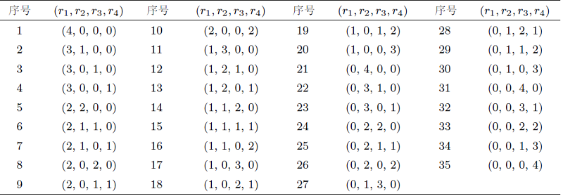
根据 4×4 RSS 过程:从排好次序的 4 个集合中分别选取 1 个个体进行测量, 则共有 $4^4$ ${\bar X_{RSS}}$ ${r_i}$ ${\mu _{(i:4)}}$ $\sigma _{(i:4)}^2$ ${r_i}$ ${r_i}$ 表1 所示.
根据定理 2.1 和表1 , 使得 $\mathrm{MSE}{({{\bar X}_{RSS}})^{({r_1},{r_2},{r_3},{r_4})}}$ $({r_1},{r_2},{r_3},{r_4}) = (r_{_1}^*,r_{_2}^*,r_{_3}^*, r_{_4}^*)$
3 可循环 4×4 最优 RSS 设计下总体均值的估计及其 MSE
为进一步提高估计的精度, 本节基于第 2 节的 4×4 最优 RSS 设计构造可循环 4×4 最优 RSS 设计下总体均值的估计, 并研究了该估计的 MSE.
令 $\left\{ {\bigcup\limits_{k = 1}^r {\left( {\bigcup\limits_{j = 1}^{r_{_1}^*} {{X_{k(1:4)j}}} \bigcup\limits_{j = 1}^{r_{_2}^*} {{X_{k(2:4)j}}} \bigcup\limits_{j = 1}^{r_{_3}^*} {{X_{k(3:4)j}}} \bigcup\limits_{j = 1}^{r_{_4}^*} {{X_{k(4:4)j}}} } \right)} } \right\}$ $X$ $4r$ ${X_{k(i:4)j}}$ $k$ $(k = 1, 2,..., r)$ $i$ $j$ ${X_{k(1:4)j}},{X_{k(2:4)j}},{X_{k(3:4)j}}$ ${X_{k(4:4)j}}$
接着, 我们给出 ${{\bar X}_{RS{S_r}}}$
定理3.1 对于可循环 4×4 最优 RSS 设计 $({r_1},{r_2},{r_3},{r_4}) = (rr_{_1}^*,rr_{_2}^*,rr_{_3}^*,rr_{_4}^*)$ ${{\bar X}_{RS{S_r}}}$
(3.1) $\begin{equation} \begin{aligned} \mathrm{MSE}{({{\bar X}_{RS{S_r}}})^{({r_1},{r_2},{r_3},{r_4})}} &= \frac{1}{{16r}}\left( {r_1^*\sigma _{(1:4)}^2 + r_2^*\sigma _{(2:4)}^2 + r_3^*\sigma _{(3:4)}^2 + r_4^*\sigma _{(4:4)}^2} \right)\\ & + {\left[ {\frac{1}{4}\left( {r_{_1}^*{\mu _{(1:4)}} + r_{_2}^*{\mu _{(2:4)}} + r_{_3}^*{\mu _{(3:4)}} + r_{_4}^*{\mu _{(4:4)}}} \right) - \mu } \right]^2}. \end{aligned} \end{equation}$
证 ${{\bar X}_{RS{S_r}}}$
4 基于 MSE 最小准则下一些分布中总体均值估计的 4×4 最优 RSS 设计
本节在表 1 给定的 4×4 RSS 设计下, 基于 MSE 最小准则找到了正态分布, 均匀分布和指数分布的 4×4 最优 RSS 设计.
例 4.1 基于 MSE 最小准则下, 寻找伴随 $\mu = 0$ ${\sigma ^2} = 1$ $N(0,1)$
因为 $N(0,1)$
(4.1) $\begin{equation} \begin{aligned} F(x) = \int_{ - \infty }^x {\frac{1}{{\sqrt {2\pi } }}{\mathrm{e}^{ - \frac{{{y^2}}}{2}}}\mathrm{d}y} \end{aligned} \end{equation}$
(4.2) $\begin{equation} \begin{aligned} f(x) = \frac{1}{{\sqrt {2\pi } }}{\mathrm{e}^{ - \frac{{{x^2}}}{2}}}, \end{aligned} \end{equation}$
接着, 把(4.1)和(4.2)式代入(2.1)-(2.4)式可得
(4.3) $\begin{equation} \begin{aligned} {f_{(1:4)}}(x) = \frac{4}{{\sqrt {2\pi } }}{\mathrm{e}^{ - \frac{{{x^2}}}{2}}}{\left( {1 - \int_{ - \infty }^x {\frac{1}{{\sqrt {2\pi } }}{\mathrm{e}^{ - \frac{{{y^2}}}{2}}}\mathrm{d}y} } \right)^3}, \end{aligned} \end{equation}$
(4.4) $\begin{equation} \begin{aligned} {f_{(2:4)}}(x) = \frac{{12}}{{\sqrt {2\pi } }}{\mathrm{e}^{ - \frac{{{x^2}}}{2}}}\left( {\int_{ - \infty }^x {\frac{1}{{\sqrt {2\pi } }}{\mathrm{e}^{ - \frac{{{y^2}}}{2}}}\mathrm{d}y} } \right){\left( {1 - \int_{ - \infty }^x {\frac{1}{{\sqrt {2\pi } }}{\mathrm{e}^{ - \frac{{{y^2}}}{2}}}\mathrm{d}y} } \right)^2}, \end{aligned} \end{equation}$
(4.5) $\begin{equation} \begin{aligned} {f_{(3:4)}}(x) = \frac{{12}}{{\sqrt {2\pi } }}{\mathrm{e}^{ - \frac{{{x^2}}}{2}}}{\left( {\int_{ - \infty }^x {\frac{1}{{\sqrt {2\pi } }}{\mathrm{e}^{ - \frac{{{y^2}}}{2}}}\mathrm{d}y} } \right)^2}\left( {1 - \int_{ - \infty }^x {\frac{1}{{\sqrt {2\pi } }}{\mathrm{e}^{ - \frac{{{y^2}}}{2}}}\mathrm{d}y} } \right) \end{aligned} \end{equation}$
(4.6) $\begin{equation} \begin{aligned} {f_{(4:4)}}(x) = \frac{4}{{\sqrt {2\pi } }}{\mathrm{e}^{ - \frac{{{x^2}}}{2}}}{\left( {\int_{ - \infty }^x {\frac{1}{{\sqrt {2\pi } }}{\mathrm{e}^{ - \frac{{{y^2}}}{2}}}\mathrm{d}y} } \right)^3}. \end{aligned} \end{equation}$
(4.7) $\begin{equation} \begin{aligned} {\mu _{(1:4)}} = \int_{ - \infty }^{ + \infty } {\frac{{4x}}{{\sqrt {2\pi } }}{\mathrm{e}^{ - \frac{{{x^2}}}{2}}}{{\left( {1 - \int_{ - \infty }^x {\frac{1}{{\sqrt {2\pi } }}{\mathrm{e}^{ - \frac{{{y^2}}}{2}}}\mathrm{d}y} } \right)}^3}} \mathrm{d}x = - 1.029375, \end{aligned} \end{equation}$
(4.8) $\begin{equation} \begin{aligned} \sigma _{(1:4)}^2 = \int_{ - \infty }^{ + \infty } {\frac{{4{x^2}}}{{\sqrt {2\pi } }}{\mathrm{e}^{ - \frac{{{x^2}}}{2}}}{{\left( {1 - \int_{ - \infty }^x {\frac{1}{{\sqrt {2\pi } }}{\mathrm{e}^{ - \frac{{{y^2}}}{2}}}\mathrm{d}y} } \right)}^3}} - \mu _{(1:4)}^2\mathrm{d}x = 0.491716109, \end{aligned} \end{equation}$
(4.9) $\begin{equation} \begin{aligned} {\mu _{(2:4)}} &= \int_{ - \infty }^{ + \infty } {\frac{{12x}}{{\sqrt {2\pi } }}{\mathrm{e}^{ - \frac{{{x^2}}}{2}}}\left( {\int_{ - \infty }^x {\frac{1}{{\sqrt {2\pi } }}{\mathrm{e}^{ - \frac{{{y^2}}}{2}}}\mathrm{d}y} } \right){{\left( {1 - \int_{ - \infty }^x {\frac{1}{{\sqrt {2\pi } }}{\mathrm{e}^{ - \frac{{{y^2}}}{2}}}\mathrm{d}y} } \right)}^2}\mathrm{d}x}\\ &= - 0.2970114, \end{aligned} \end{equation}$
(4.10) $\begin{equation} \begin{aligned} \sigma _{(2:4)}^2 &= \int_{ - \infty }^{ + \infty } {\frac{{12{x^2}}}{{\sqrt {2\pi } }}{\mathrm{e}^{ - \frac{{{x^2}}}{2}}}\left( {\int_{ - \infty }^x {\frac{1}{{\sqrt {2\pi } }}{\mathrm{e}^{ - \frac{{{y^2}}}{2}}}\mathrm{d}y} } \right){{\left( {1 - \int_{ - \infty }^x {\frac{1}{{\sqrt {2\pi } }}{\mathrm{e}^{ - \frac{{{y^2}}}{2}}}\mathrm{d}y} } \right)}^2}} - \mu _{(2:4)}^2\mathrm{d}x\\ &= 0.360455328, \end{aligned} \end{equation}$
(4.11) $\begin{equation} \begin{aligned} {\mu _{(3:4)}} &= \int_{ - \infty }^{ + \infty } {\frac{{12x}}{{\sqrt {2\pi } }}{\mathrm{e}^{ - \frac{{{x^2}}}{2}}}{{\left( {\int_{ - \infty }^x {\frac{1}{{\sqrt {2\pi } }}{\mathrm{e}^{ - \frac{{{y^2}}}{2}}}\mathrm{d}y} } \right)}^2}\left( {1 - \int_{ - \infty }^x {\frac{1}{{\sqrt {2\pi } }}{\mathrm{e}^{ - \frac{{{y^2}}}{2}}}\mathrm{d}y} } \right)\mathrm{d}x}\\ &= 0.2970114, \end{aligned} \end{equation}$
(4.12) $\begin{equation} \begin{aligned} \sigma _{(3:4)}^2 &= \int_{ - \infty }^{ + \infty } {\frac{{12{x^2}}}{{\sqrt {2\pi } }}{\mathrm{e}^{ - \frac{{{x^2}}}{2}}}{{\left( {\int_{ - \infty }^x {\frac{1}{{\sqrt {2\pi } }}{\mathrm{e}^{ - \frac{{{y^2}}}{2}}}\mathrm{d}y} } \right)}^2}\left( {1 - \int_{ - \infty }^x {\frac{1}{{\sqrt {2\pi } }}{\mathrm{e}^{ - \frac{{{y^2}}}{2}}}\mathrm{d}y} } \right)} - \mu _{(3:4)}^2\mathrm{d}x\\ &= 0.360455328, \end{aligned} \end{equation}$
(4.13) $\begin{equation} \begin{aligned} {\mu _{(4:4)}} = \int_{ - \infty }^{ + \infty } {\frac{{4x}}{{\sqrt {2\pi } }}{\mathrm{e}^{ - \frac{{{x^2}}}{2}}}{{\left( {\int_{ - \infty }^x {\frac{1}{{\sqrt {2\pi } }}{\mathrm{e}^{ - \frac{{{y^2}}}{2}}}\mathrm{d}y} } \right)}^3}\mathrm{d}x} = 1.029375 \end{aligned} \end{equation}$
(4.14) $\begin{equation} \begin{aligned} \sigma _{(4:4)}^2 = \int_{ - \infty }^{ + \infty } {\frac{{4{x^2}}}{{\sqrt {2\pi } }}{\mathrm{e}^{ - \frac{{{x^2}}}{2}}}{{\left( {\int_{ - \infty }^x {\frac{1}{{\sqrt {2\pi } }}{\mathrm{e}^{ - \frac{{{y^2}}}{2}}}\mathrm{d}y} } \right)}^3}} - \mu _{(4:4)}^2\mathrm{d}x = 0.491716109. \end{aligned} \end{equation}$
当 $({r_1},{r_{_2}},{r_3},{r_4}) = (2,2,0,0)$
接着, 其它 RSS 设计依次由定理 2.1 计算可得 MSE 数值结果如表2 所示.
因此, 由表2 可知基于 MSE 最小准则下, $N(0,1)$
例 4.2 基于 MSE 最小准则下, 寻找伴随 $\mu = \frac{1}{2}$ ${\sigma ^2} = \frac{1}{{12}}$ $U(0,1)$
因为 $U(0,1)$ $F(x)=x$ $f(x)=1$
(4.15) $\begin{equation} \begin{aligned} {f_{(1:4)}}(x) = 4{(1 - x)^3}, \end{aligned} \end{equation}$
(4.16) $\begin{equation} \begin{aligned} {f_{(2:4)}}(x) = 12x{(1 - x)^2}, \end{aligned} \end{equation}$
(4.17) $\begin{equation} \begin{aligned} {f_{(3:4)}}(x) = 12{x^2}(1 - x) \end{aligned} \end{equation}$
(4.18) $\begin{equation} \begin{aligned} {f_{(4:4)}}(x) = 4{x^3}. \end{aligned} \end{equation}$
(4.19) $\begin{equation} \begin{aligned} {\mu _{(1:4)}} = \int_0^1 {4x{{(1 - x)}^3}} \mathrm{d}x = 0.2, \end{aligned} \end{equation}$
(4.20) $\begin{equation} \begin{aligned} \sigma _{(1:4)}^2 = \int_0^1 {4{x^2}{{(1 - x)}^3}} - \mu _{(1:4)}^2\mathrm{d}x = 0.026666667, \end{aligned} \end{equation}$
(4.21) $\begin{equation} \begin{aligned} {\mu _{(2:4)}} = \int_0^1 {12{x^2}{{(1 - x)}^2}} \mathrm{d}x = 0.4, \end{aligned} \end{equation}$
(4.22) $\begin{equation} \begin{aligned} \sigma _{(2:4)}^2 = \int_0^1 {12{x^3}{{(1 - x)}^2}} - \mu _{(2:4)}^2\mathrm{d}x = 0.04, \end{aligned} \end{equation}$
(4.23) $\begin{equation} \begin{aligned} {\mu _{(3:4)}} = \int_0^1 {12{x^3}(1 - x)} \mathrm{d}x = 0.6, \end{aligned} \end{equation}$
(4.24) $\begin{equation} \begin{aligned} \sigma _{(3:4)}^2 = \int_0^1 {12{x^4}(1 - x)} - \mu _{(3:4)}^2\mathrm{d}x = 0.04, \end{aligned} \end{equation}$
(4.25) $\begin{equation} \begin{aligned} {\mu _{(4:4)}} = \int_0^1 {4{x^4}} \mathrm{d}x = 0.8 \end{aligned} \end{equation}$
(4.26) $\begin{equation} \begin{aligned} \sigma _{(4:4)}^2 = \int_0^1 {4{x^5}} - \mu _{(4:4)}^2\mathrm{d}x = 0.026666667. \end{aligned} \end{equation}$
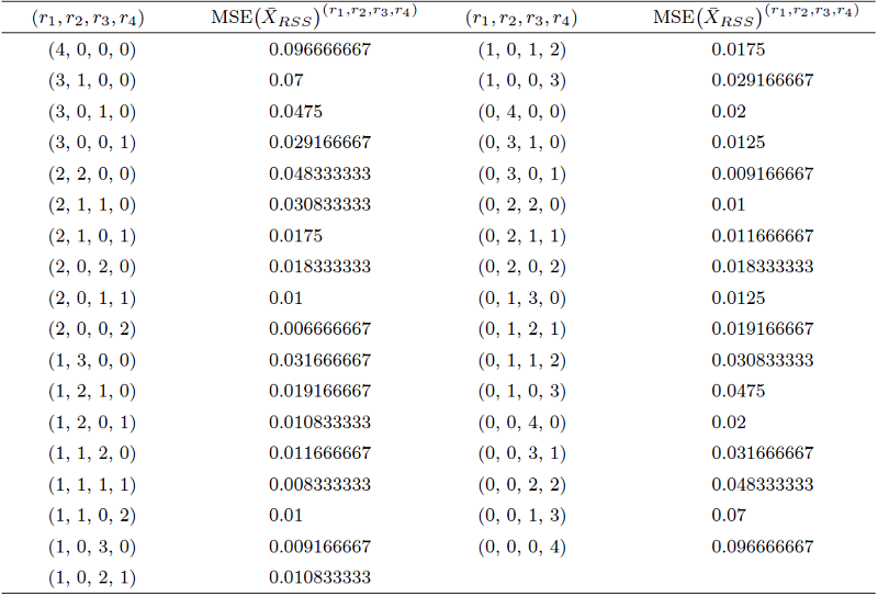
当 $({r_1},{r_{_2}},{r_3},{r_4}) = (3,0,1,0)$
接着, 其它 RSS 设计依次由定理 2.1 计算可得 MSE 数值结果如表3 所示.
因此, 由表3 可知基于 MSE 最小准则下, $U(0,1)$
例 4.3 基于 MSE 最小准则下, 寻找伴随 $\mu = 1$ ${\sigma ^2} = 1$ $(1)$
因为 $\mathrm{Exp}(1)$ $F(x) = 1 - {\mathrm{e}^{ - x}}$ $f(x) = {\mathrm{e}^{ - x}}$
(4.27) $\begin{equation} \begin{aligned} {f_{(1:4)}}(x) = 4{\mathrm{e}^{ - 4x}}, \end{aligned} \end{equation}$
(4.28) $\begin{equation} \begin{aligned} {f_{(2:4)}}(x) = 12(1 - {\mathrm{e}^{ - x}}){\mathrm{e}^{ - 3x}}, \end{aligned} \end{equation}$
(4.29) $\begin{equation} \begin{aligned} {f_{(3:4)}}(x) = 12{(1 - {\mathrm{e}^{ - x}})^2}{\mathrm{e}^{ - 2x}} \end{aligned} \end{equation}$
(4.30) $\begin{equation} \begin{aligned} {f_{(4:4)}}(x) = 4{(1 - {\mathrm{e}^{ - x}})^3}{\mathrm{e}^{ - x}}. \end{aligned} \end{equation}$
(4.31) $\begin{equation} \begin{aligned} {\mu _{(1:4)}} = \int_0^{ + \infty } {4x{\mathrm{e}^{ - 4x}}} \mathrm{d}x = 0.25, \end{aligned} \end{equation}$
(4.32) $\begin{equation} \begin{aligned} \sigma _{(1:4)}^2 = \int_0^{ + \infty } {4{x^2}{\mathrm{e}^{ - 4x}}} - \mu _{(1:4)}^2\mathrm{d}x = 0.0625, \end{aligned} \end{equation}$
(4.33) $\begin{equation} \begin{aligned} {\mu _{(2:4)}} = \int_0^{ + \infty } {12x(1 - {\mathrm{e}^{ - x}}){\mathrm{e}^{ - 3x}}} \mathrm{d}x = 0.583333333, \end{aligned} \end{equation}$
(4.34) $\begin{equation} \begin{aligned} \sigma _{(2:4)}^2 = \int_0^{ + \infty } {12{x^2}(1 - {\mathrm{e}^{ - x}}){\mathrm{e}^{ - 3x}}} - \mu _{(2:4)}^2\mathrm{d}x = 0.173611161, \end{aligned} \end{equation}$
(4.35) $\begin{equation} \begin{aligned} {\mu _{(3:4)}} = \int_0^{ + \infty } {12x{{(1 - {\mathrm{e}^{ - x}})}^2}{\mathrm{e}^{ - 2x}}} \mathrm{d}x = 1.083333333, \end{aligned} \end{equation}$
(4.36) $\begin{equation} \begin{aligned} \sigma _{(3:4)}^2 = \int_0^{ + \infty } {12{x^2}{{(1 - {\mathrm{e}^{ - x}})}^2}{\mathrm{e}^{ - 2x}}} - \mu _{(3:4)}^2\mathrm{d}x = 0.423611611, \end{aligned} \end{equation}$
(4.37) $\begin{equation} \begin{aligned} {\mu _{(4:4)}} = \int_0^{ + \infty } {4x{{(1 - {\mathrm{e}^{ - x}})}^3}{\mathrm{e}^{ - x}}} \mathrm{d}x = 2.083333333 \end{aligned} \end{equation}$
(4.38) $\begin{equation} \begin{aligned} \sigma _{(4:4)}^2 = \int_0^{ + \infty } {4{x^2}{{(1 - {\mathrm{e}^{ - x}})}^3}{\mathrm{e}^{ - x}}} - \mu _{(4:4)}^2\mathrm{d}x = 1.423612611. \end{aligned} \end{equation}$
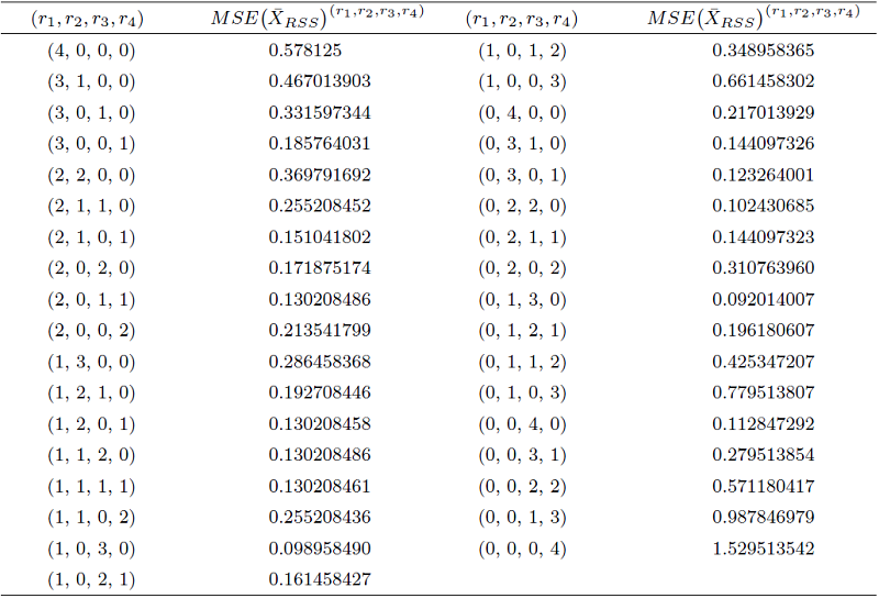
当 $({r_1},{r_{_2}},{r_3},{r_4}) = (2,1,1,0)$
接着, 其它 RSS 设计依次由定理 2.1 计算可得 MSE 数值结果如表4 所示.
因此, 由表4 可知基于 MSE 最小准则下, $Exp(1)$
5 可循环 4×4 最优 RSS 设计下一些分布中 ${{\bar X}_{RS{S_r}}}$
本节根据第 4 节中正态分布, 均匀分布和指数分布找到的 4×4 最优 RSS 设计, 基于第 3 节的理论, 计算了 ${{\bar X}_{RS{S_r}}}$
例 5.1 在可循环 4×4 最优 RSS 设计 $(r_1,r_2,r_3,r_4) = (0,2r,2r,0)$ $N(0,1)$ ${{\bar X}_{RS{S_r}}}$
(5.1) $\begin{equation} \begin{aligned} \mathrm{MSE}{({{\bar X}_{RS{S_r}}})^{(0,2r,2r,0)}} &= \frac{1}{{16r}}\left( {2\sigma _{(2:4)}^2 + 2\sigma _{(3:4)}^2} \right) + {\left[ {\frac{1}{4}\left( {2{\mu _{(2:4)}} + 2{\mu _{(3:4)}}} \right) - 0} \right]^2}\\ &= \frac{{0.090113832}}{r}. \end{aligned} \end{equation}$
由(5.1)式知, 随着 $r$ ${{\bar X}_{RS{S_r}}}$
例 5.2 在可循环 4×4 最优 RSS 设计 $(r_1,r_2,r_3,r_4) = (2r,0,0,2r)$ $U(0,1)$ ${{\bar X}_{RS{S_r}}}$
把(4.19), (4.20), (4.25), (4.260式代入(3.1)式可得
(5.2) $\begin{equation} \begin{aligned} \mathrm{MSE}{({{\bar X}_{RS{S_r}}})^{(2r,0,0,2r)}} &= \frac{1}{{16r}}\left( {2\sigma _{(1:4)}^2 + 2\sigma _{(4:4)}^2} \right) + {\left[ {\frac{1}{4}\left( {2{\mu _{(1:4)}} + 2{\mu _{(4:4)}}} \right) - \frac{1}{2}} \right]^2}\\ &= \frac{{0.006666667}}{r}. \end{aligned} \end{equation}$
由(5.2)式知, 随着 $r$ ${{\bar X}_{RS{S_r}}}$
例 5.3 在可循环 4×4 最优 RSS 设计 $(r_1,r_2,r_3,r_4) = (0,r,3r,0)$ $(1)$ ${{\bar X}_{RS{S_r}}}$
(5.3) $\begin{equation} \begin{aligned} \mathrm{MSE}{({{\bar X}_{RS{S_r}}})^{(0,r,3r,0)}} &= \frac{1}{{16r}}\left( {\sigma _{(2:4)}^2 + 3\sigma _{(3:4)}^2} \right) + {\left[ {\frac{1}{4}\left( {{\mu _{(2:4)}} + 3{\mu _{(3:4)}}} \right) - 1} \right]^2}\\ &= \frac{{0.090277875}}{r} + 0.001736133. \end{aligned} \end{equation}$
由(5.3)式知, 随着 $r$ ${{\bar X}_{RS{S_r}}}$
6 结语
本文给出了 4×4 RSS 设计下总体均值估计的 MSE 及其 35 种设计. 基于 MSE 最小准则下, 给出了寻找总体均值估计的 4×4 最优 RSS 设计的一般结论, 然后研究了可循环 4×4 最优 RSS 设计下 ${{\bar X}_{RS{S_r}}}$
针对正态分布, 均匀分布和指数分布, 本文基于 MSE 最小准则下, 找到了这三个分布总体均值估计的 4×4 最优 RSS 设计, 并进一步研究了这三个分布在可循环 4×4 最优 RSS 设计下 ${{\bar X}_{RS{S_r}}}$ ${{\bar X}_{RS{S_r}}}$
有如下问题值得进一步的研究. 第一, 本文考虑了 MSE 最小准则下总体均值估计的 4×4 最优 RSS 设计及其性质, 如何在 MSE 最小准则下, 获得总体均值估计的 $S$ $S$ $(S=5,6,7)$
参考文献
View Option
[1]
McIntyre G A A method for unbiased selective sampling using ranked sets
Australian Journal of Agricultural Research , 1952 , 3 4 ): 385 -390
DOI:10.1071/AR9520385
URL
[本文引用: 1]
[2]
Yang R Chen W X Maximum likelihood estimator of the shape parameter under simple random sampling and moving extremes ranked set sampling
Statistics andProbability Letters , 2025 , 226 110465
[本文引用: 1]
[3]
Dai W C Chen W X Zhao H L Estimation of the population mean under imperfect simple Z ranked set sampling
Statistical Papers , 2025 , 66 4 ): 81
DOI:10.1007/s00362-025-01707-9
[4]
Chen M Chen W X Deng C H Some new results on parameter estimation of the exponential-Poisson distribution in ranked set sampling
Applied Mathematics-A Journal of Chinese Universities Series B , 2025 , 40 2 ): 413 -428
[5]
汪寒 , 陈望学 . Bilal 分布中参数的修正极大似然估计及其抽样性质
系统科学与数学 , 2025 , 45 2 ): 639 -650
DOI:10.12341/jssms23681
Bilal分布作为寿命模型, 在生存分析中起着重要作用.文章分别在简单随机抽样(SRS)和排序集抽样(RSS)下研究了Bilal分布中参数$\theta$的修正极大似然估计(MLE),获得了该修正MLE的有限样本性质和大样本性质. 数值结果表明,同等样本容量下的RSS修正MLE比SRS修正MLE有效.数值模拟也显示同种抽样下MLE 的均方误差和修正MLE的方差是非常接近的,但具有显性解的修正MLE在实际中使用更方便.
Wang H Chen W X Modified maximum likelihood estimator and sampling properties of estimator for Bilal distribution
Journal of Systems Science and Mathematical Sciences , 2025 , 45 2 ): 639 -650
DOI:10.12341/jssms23681
Bilal distribution is the most exploited distribution for life-time data analysis. In this paper, we study the modified maximum likelihood estimator (MLE) of the parameter $\theta$ for Bilal distribution under simple random sampling (SRS) and ranked set sampling (RSS) and obtain finite sample properties and large sample properties of the modified MLE. Numerical results show that modified MLE under RSS can be real competitors against the ones based on SRS, when the sample size is used. Numerical results also show that the mean square error of classical MLE is very close to the variance of modified MLE under the same sampling, but modified MLE with explicit solution is more convenient to use in practice.
[6]
姜杰 , 陈望学 , 汪寒 . 不同类型排序集抽样设计下 Topp-Leone 分布中参数的极大似然估计及其性质
应用数学学报 , 2025 , 48 2 ): 294 -304
DOI:10.20142/j.cnki.amas.202401043
[本文引用: 1]
在统计推断里, 参数估计的好坏很大程度上依赖于抽样设计, 所以有效的抽样设计将是一项重要的研究课题. 本文分别在排序集抽样(RSS), 非均等最大值排序集抽样(MaxRSSU)和非均等最小值排序集抽样(MinRSSU)下研究了Topp-Leone分布中参数的极大似然估计(MLE)及其性质. 上述MLE渐近效率的理论结果表明MaxRSSU估计和简单随机抽样估计一样有效, RSS估计和MinRSSU估计都比简单随机抽样估计有效.
Jiang J Chen W X Wang H Maximum likelihood estimator of the parameter of Topp-Leone distribution and its properties under different types of ranked set sampling
Acta Mathematicae Applicatae Sinica , 2025 , 48 2 ): 294 -304
DOI:10.20142/j.cnki.amas.202401043
[本文引用: 1]
In statistical parameter estimation problems, how well the parameters are estimated largely depends on the sampling design used. In this article, we consider maximum likelihood estimator(MLE) of the parameter of Topp-Leone distribution and its properties under ranked set sampling(RSS), maximum ranked set sampling with unequal samples(MaxRSSU) and minimum ranked set sampling with unequal samples(MinRSSU). Theoretical results of asymptotic efficiencies of the above MLE show that the MaxRSSU estimator and the simple random sampling estimator have the same efficiency, the RSS estimator and the MinRSSU estimator are more efficient than the simple random sampling estimator.
[7]
Takahasi K Wakimoto K On unbiased estimates of the population mean based on the sample stratified by means of ordering
Annals of the Institute of Statistical Mathematics , 1968 , 20 1 ): 1 -31
DOI:10.1007/BF02911622
URL
[本文引用: 1]
[8]
Chen Z H Bai Z D Ranked Set Sampling:Theory and Applications . New York : Springer , 2004
[本文引用: 1]
[9]
Kaur A Patil G P Taillie C Unequal allocation models for ranked set sampling with skew distributions
Biometrics , 1997 , 53 123 -130
DOI:10.2307/2533102
URL
[本文引用: 1]
[10]
Chen W X Tian Y Xie M Y Maximum likelihood estimator of the parameter for a continuous one-parameter exponential family under the optimal ranked set sampling
Journal of Systems Science and Complexity , 2017 , 30 6 ): 128 -141
[11]
Chen W X Tian Y Xie M Y The global minimum variance unbiased estimator of the parameter for a truncated parameter family under the optimal ranked set sampling
Journal of Statistical Computation and Simulation , 2018 , 88 17 ): 3399 -3414
DOI:10.1080/00949655.2018.1520233
URL
[12]
张棚 , 陈望学 . 最优排序集抽样下正态分布中总体方差的优良估计及其性质
系统科学与数学 , 2026 , 46 6 ): 2048 -2063
DOI:10.12341/jssms240884
文章在平衡排序集抽样 (RSS) 设计下研究了 $N(\mu,{\sigma ^2})$ 分布中 $\mu$ 已知时, 总体方差 ${\sigma ^2}$ 的优良估计及其性质. 理论结果表明, 总体方差的平衡 RSS 估计比简单随机抽样 (SRS) 估计有效. 为进一步提高统计推断的效率, 文章提出了适用于该模型的 Fisher 信息量最大化 RSS 设计和拟充分完全统计量 RSS 设计, 并在这两种设计下研究了该模型中总体方差的优良估计及其性质. 研究结果表明, 总体方差的 Fisher 信息量最大化 RSS 估计和拟充分完全统计量 RSS 估计都比平衡 RSS 估计有效. 总体方差的拟充分完全统计量 RSS 估计比 Fisher 信息量最大化 RSS 估计有效. 另外,文章在平衡 RSS 下研究了 $N(\mu,{\sigma ^2})$ 分布中 $\mu$ 未知时, 总体方差 ${\sigma ^2}$ 的优良估计及其性质. 研究结果表明, $\mu$ 未知时总体方差的平衡 RSS 估计比 SRS 估计有效. 实际数据分析进一步验证了这个研究结果.
Zhang P Chen W X Some properties of optimal estimation of population variance for normal distribution under optimal ranked set sampling
Journal of Systems Science and Mathematical Sciences , 2026 , 46 6 ): 2048 -2063
DOI:10.12341/jssms240884
This paper explores the characteristics of optimal estimation for the population variance $\sigma ^2$ in a normal distribution $N(\mu,{\sigma ^2})$, where $\mu$ is known, utilizing balanced ranked set sampling (RSS). The theoretical findings indicate that the balanced RSS estimation of population variance exhibits greater efficiency compared to the estimation derived from simple random sampling (SRS). To enhance the efficiency of statistical inference, we propose a Fisher information maximization approach and a quasi-sufficient complete statistic framework for the RSS design. Furthermore, we investigate the optimal estimation of population variance and analyze its characteristics under these two methodologies. The numerical findings indicate that the RSS estimation of population variance utilizing Fisher information maximization, as well as the RSS estimation based on quasi-sufficient complete statistics, exhibit superior efficiency compared to the balanced RSS estimation. Furthermore, the quasi-sufficient complete statistic RSS estimation for population variance demonstrates greater efficiency than that derived from Fisher information maximization. Furthermore, this paper explores the characteristics of optimal estimation for the population variance $\sigma ^2$ in a normal distribution $N(\mu,{\sigma ^2})$, where $\mu$ is unknown, utilizing balanced RSS. The numerical findings indicate that the balanced RSS estimation of population variance exhibits greater efficiency compared to the estimation derived from SRS when $\mu$ is unknown. The real data analysis is provided to illustrate the numerical findings.
[13]
Li M M Chen W X $3$ $3$ $k$
Statistics and Probability Letters , 2025 , 224 110455
[本文引用: 1]
[14]
Al-Saleh M F Steady-state ranked set sampling and parametric estimation
Journal of Statistical Planning and Inference , 2004 , 123 1 ): 83 -95
DOI:10.1016/S0378-3758(03)00139-3
URL
[本文引用: 2]
A method for unbiased selective sampling using ranked sets
1
1952
... 排序集抽样 (Ranked set sampling, RSS )是一种试图用来提高抽样效率的方法, 由澳大利亚农业学家 McIntyre[1 ] 在估计农场牧草产量均值时提出, 近年来已得到了广泛的研究和应用, 见文献[2 6 ]. RSS 适用于那些对所研究的变量进行精确测量既困难又耗时漫长, 但是在一个相对小的集合中可以通过非精确测量手段进行排序的场合. ...
Maximum likelihood estimator of the shape parameter under simple random sampling and moving extremes ranked set sampling
1
2025
... 排序集抽样 (Ranked set sampling, RSS )是一种试图用来提高抽样效率的方法, 由澳大利亚农业学家 McIntyre[1 ] 在估计农场牧草产量均值时提出, 近年来已得到了广泛的研究和应用, 见文献[2 6 ]. RSS 适用于那些对所研究的变量进行精确测量既困难又耗时漫长, 但是在一个相对小的集合中可以通过非精确测量手段进行排序的场合. ...
Estimation of the population mean under imperfect simple Z ranked set sampling
0
2025
Some new results on parameter estimation of the exponential-Poisson distribution in ranked set sampling
0
2025
Bilal 分布中参数的修正极大似然估计及其抽样性质
0
2025
Modified maximum likelihood estimator and sampling properties of estimator for Bilal distribution
0
2025
不同类型排序集抽样设计下 Topp-Leone 分布中参数的极大似然估计及其性质
1
2025
... 排序集抽样 (Ranked set sampling, RSS )是一种试图用来提高抽样效率的方法, 由澳大利亚农业学家 McIntyre[1 ] 在估计农场牧草产量均值时提出, 近年来已得到了广泛的研究和应用, 见文献[2 6 ]. RSS 适用于那些对所研究的变量进行精确测量既困难又耗时漫长, 但是在一个相对小的集合中可以通过非精确测量手段进行排序的场合. ...
Maximum likelihood estimator of the parameter of Topp-Leone distribution and its properties under different types of ranked set sampling
1
2025
... 排序集抽样 (Ranked set sampling, RSS )是一种试图用来提高抽样效率的方法, 由澳大利亚农业学家 McIntyre[1 ] 在估计农场牧草产量均值时提出, 近年来已得到了广泛的研究和应用, 见文献[2 6 ]. RSS 适用于那些对所研究的变量进行精确测量既困难又耗时漫长, 但是在一个相对小的集合中可以通过非精确测量手段进行排序的场合. ...
On unbiased estimates of the population mean based on the sample stratified by means of ordering
1
1968
... Takahasi 和 Wakimoto[7 ] 建立了 RSS 的数学理论基础, 并证明了平衡 RSS 下用样本均值作为总体均值的估计比简单随机抽样 (Simple Ranked Set Sampling, SRS )用样本均值作为总体均值的估计更有效. ...
1
2004
... 因为排序不经过测量, 所以合理选择 RSS 的集合大小 $m$ [8 ] 指出集合大小 $m$
Unequal allocation models for ranked set sampling with skew distributions
1
1997
... 平衡 RSS 适用于总体分布完全未知时的统计推断, 但如果已有总体分布的某些信息时, 使用某些准则就可以进一步提高统计推断的效率, 见文献[9 13 ]. ...
Maximum likelihood estimator of the parameter for a continuous one-parameter exponential family under the optimal ranked set sampling
0
2017
The global minimum variance unbiased estimator of the parameter for a truncated parameter family under the optimal ranked set sampling
0
2018
最优排序集抽样下正态分布中总体方差的优良估计及其性质
0
2026
Some properties of optimal estimation of population variance for normal distribution under optimal ranked set sampling
0
2026
$3$ ×$3$ optimal ranked set sampling design with $k$ cycles and best linear invariant estimators of the parameters for normal distribution
1
2025
... 平衡 RSS 适用于总体分布完全未知时的统计推断, 但如果已有总体分布的某些信息时, 使用某些准则就可以进一步提高统计推断的效率, 见文献[9 13 ]. ...
Steady-state ranked set sampling and parametric estimation
2
2004
... Al-Saleh[14 ] 在均方误差 (MSE )最小准则下, 针对正态分布、均匀分布和指数分布找到了总体均值估计的 3×3 最优 RSS 设计. ...
... 本文在文献[14 ] 的基础上, 基于 MSE 最小准则下, 针对正态分布、均匀分布和指数分布找到了总体均值估计的 4×4 最优 RSS 设计. 为了进一步提高估计的精度, 本文研究了这些分布在可循环 4×4 最优 RSS 设计下总体均值估计的 MSE, 研究结果表明在可循环 4×4 最优 RSS 设计下这些分布中总体均值估计的 MSE 随着循环的增大不断减小. ...