神经网络作为处理复杂问题的有效工具, 在模式识别, 参数优化, 联想记忆与信号处理^[1,2,3,4] 等领域取得了广泛应用. 相较于仅存在单一全局稳定平衡点的单稳定性系统, 多稳定性系统在有限状态空间内存在多个局部稳定平衡点. 这一特性使得多平衡点的存在性验证与稳定性分析往往更具挑战性. 而且, 多平衡点的数目和位置与神经网络的存储和检索能力密切相关, 是模式识别与联想记忆等领域最重要的性能指标. 因此神经网络多稳定性的研究得到了广泛关注, 如文献[5] 讨论了具有不连续, 非单调, 分段且非线性激活函数的神经网络多稳定性, 文献[6] 则关注到无界时变延迟和周期激活函数对递归神经网络多稳定性的影响, 更多的神经网络多稳定性方向的研究工作可见参考文献[7,8,9,10].

作为一类广义递归神经网络, Cohen-Grossberg 神经网络自从在文献[11] 中被提出, 其优越的性能就得到了广泛关注, 如多种时延影响下的稳定性分析^[12,13,14],

鲁棒性分析^[15]和渐近周期解^[16]. 此外, 文献[17] 讨论了混合时延影响下的 Cohen-Grossberg 神经网络的多模态稳定, 而文献[18] 研究了基于忆阻器的 Cohen-Grossberg 神经网络的多稳定性, 这为不连续的 Cohen-Grossberg 神经网络的稳定性研究提供了一个新的思路.

相比较于传统的整数阶微积分, 分数阶微积分可以更精确地描述实际演变过程. 换而言之, 利用分数阶微积分构造的动力学方程在物理系统, 工程系统与自动控制系统的建模中具有更高的建模精度. 这是因为分数微积分的记忆特性可以更好的描述时间内状态的总体行为. 这促使许多研究工作探讨了分数阶神经网络的多种动态行为, 如单稳定性与多稳定性^[19], 多重渐近稳定性, $S$-渐近 $\omega$ 周期^[20,21], Mittag-Leffler

输入稳定性^[22]与预定时间同步^[23]. 更多的分数阶 Cohen-Grossberg 神经网络的多稳定性的相关研究参见文献[24,25,26]. 需要注意的是上述参考文献中都没有考虑到切换在神经网络动态行为中的作用.

众所周知, 在工程, 化学, 生物医学等诸多领域中存在着许多具有状态依赖切换的系统, 如基于忆阻器的神经网络, 其连接权值会随着状态的变化而发生跳变. 而切换点的存在可能会增加平衡点的数目, 这代表着神经网络的存储容量和检索能力都会进一步得到增强^[27], 因此对切换神经网络的研究工作是很有必要的. 如何结合状态依赖切换神经网络和分数阶神经网络的优点, 激发了很多研究者的热情,

如文献[28,29,30]分别考虑 Sigmoidal 函数与 Gaussian 函数作为激活函数时, 状态依赖切换对于分数阶神经网络多稳定性的影响.

值得注意的是, 上述文献均没有考虑到时延的问题. 在神经网络中时延一般表现为神经元的延迟激活, 这种异常激活会导致神经网络的非线性震荡乃至失稳. 文献[31,32]在递归神经网络中考虑了时延的影响, 分析了具有分段线性激活函数和 Sigmoidal 激活参数时的多稳定性. 现有的递归神经网络和 Hopfield 神经网络在结构上与 Cohen-Grossberg 神经网络相似, 均可视为 Cohen-Grossberg 神经网络中具有不同参数的一种特殊情况, 但关于具有时变时延和状态依赖切换的 Cohen-Grossberg 神经网络的多稳定性的研究较为稀少.

经由上述讨论, 本文研究的是具有时变时延与状态依赖切换的分数阶 Cohen-Grossberg 神经网络的多稳定性问题. 主要贡献概述如下, 首先本文考虑的分数阶系统中同时考虑的切换问题与时延问题更具一般性, 这是因为具有状态依赖的参数切换与时变时延的神经网络在实际工程问题中有着更广的适用范围. 其次, 本文使用状态空间划分的方法研究了 SFCGNNs, 所得到的推导结果包含了 Hopfield 神经网络与递归神经网络的研究结果. 第三, 利用 Brouwer's 不动点定理, 微分包含理论与 Lyapunov 稳定性理论, 给出了 SFCGNNs 具有 $5^n$ 个平衡点的充分条件, 其中 $3^n$ 个平衡点是渐近稳定的, 其余平衡点则是不稳定的. 相比较于前人的成果, 本文的结果是新的, 且更具一般性, 是对前人所做工作的概括与拓展.

本文其余内容结构如下: 在第 2 节中, 将介绍 SFCGNNs 的模型描述, 分数阶导数的定义与一些其他的预备知识; 第 3 节中, 利用状态空间划分的方法与分数阶 Caputo 导数分别推到了推导出了保证 SFCGNNs 具有 $5^n$ 个平衡点的充分条件, 证明了 $3^n$ 个平衡点是渐近稳定的, 同时也给出了其余的 $5^n-3^n$ 个平衡点不稳定的充分条件; 第 4 节中, 结合两个数值算例验证结果的有效性; 最后, 第 5 节是对本文的研究内容进行的总结.

考虑具有状态依赖切换的分数阶 Cohen-Grossberg 神经网络, 下面是其分数阶微分方程:

此处 $x=(x_1,x_2,\cdots,x_n)^T$ 是状态向量, $I_{i}$ 表示外部输入, $t_\tau=t+\tau(t)$, 其中 $\tau(t)$ 表示延迟时间, 且有 $-\tau\le \tau(t) <0$. $\alpha_{i}(x_{i}(t))$ 是增益, $\mu_{i}(x_{i}(t))$ 是自抑制函数, 且满足 $\alpha_{i}^{'}$, $\alpha_{i}^{''}$, $\mu _{i}^{'}$ 与 $\mu_{i}^{''}$ 均为大于 0 的常数. $\delta_{ij}(x_{j}(t))$ 与 $\rho_{ij}(x_{j}(t_\tau))$ 是连接权值, 其中 $\delta _{i}^{'}, \delta _{ij}^{''}, \rho _{ij}^{'}, \rho _{ij}^{''}$ 均为常数. 本文所讨论的是具有状态依赖的绝对值切换, 即当系统状态的绝对值达到阈值时系统参数会发生切换, 对于切换跳变 $\mathcal{K}_i>0,\mathcal{K}_j>0$ 满足以下切换规则:

系统(2.1)的初值定义为 $x_i(s) =\phi _i(s-t_0),s\in[t_0-\tau,t_0],\phi\in C((-\tau,0],\Re)$. 并且其中激活函数满足以下假设:

假设 1: 激活函数 $ \mathcal{G}_i$ 是连续函数具有饱和区间, 即存在两个常数 $m_{i}$ 与 $M_{i}$ 使得 $\lim_{u\rightarrow+\infty}G_{i}(u)=M_{i}$, $\lim_{u\rightarrow -\infty}G_{i}(u)=m_{i} $.

假设 2: 对于 $\forall u\in \Re$, 存在正常数 $k_i$, 使得 $0<\mathcal{G}_{i}^{'}(u)\le k_i$, 在此基础上若有 $u\ne 0$, 则 $u\mathcal{G}_{i}^{''}(u) <0$. 记 $\check{k}_i=\sup_{|u|\geq \mathcal{K}_i}\mathcal{G}_{i}^{'}(u)$, $ k_i=\sup_{|u|<\mathcal{K}_i}\mathcal{G}_{i}^{'}(u)$.

定义 $\Re ^n$ 是 n 维实空间. 向量 $ v=(v_1,v_2,\cdots,v_n )^T\in \Re ^n$ 是一个列向量. 定义 $C^n((t_0,+\infty),\Re^n) $ 是将 $(t_0,+\infty)$ 区间映射到 $\Re^n$ 的 n 次连续函数映射. $[\cdot,\cdot] $ 是代表区间, co$ [a,b] $ 表示由实数 $a, b$ 构成的闭凸包, 同样的 co$[\omega]$ 代表由给定集合 $\omega$ 构成的凸包, 其中 $\omega \in \Re$. 符号 $\mathcal{D}^{q} h_{i}(t)$ 与 $\mathcal{I}^{q}h_{i}(t)$ 分别表示 $h_{i}(t)$ 的阶数为 $q$ 的 Caputo 分数阶导数与分数阶积分. 另外, 本篇论文所考虑的所有系统的解均为 Filippov 意义下的解.

对于 SFCGNNs (2.1), 考虑如下集值映射

通过微分包含理论, 根据 SFCGNNs (2.1), 对于 $i \in 1,\ldots,n$

定义 2.1 (^[33]) 列向量 $ x(t) = \left( x_1(t), \ldots, x_n(t) \right)^T$ 是 SFCGNNs (1) 具有初值 $ x_i\left( s \right) =\phi _i\left( s-t_0 \right),s\in \left[ t_0-\tau,t_0 \right] $ 的 Filippov 解, 如果对于 $ \forall i \in \left(1, \ldots, n \right) $, 有 $ x_i(t) $ 在 $ t \in [0, +\infty) $ 的任意闭区间上绝对连续并且满足以下微分包含

定义 2.2 (^[33]) 常数列向量 $ x^*=\left(x^*_{1}, \ldots, x^*_{n}\right)^{T}$ 可以被称为 SFCGNNs (1) 的平衡点, 如果 $\forall i \in \mathbb{N} $, $ x^*_{i} $ 满足

引理 2.1 (^[34]) 如果 $ y\left( t \right) \in \Re ^n $ 可微, $ q\in \left( 0,1 \right] $, 而且 Q 是正定的, 那么

引理 2.2 (^[35]) 假设 $ 0<q<1 $ 并且 $ h(t) $ 是可微的, 如果存在一些时刻 $ 0<t<t_1 $ 使得 $ h\left( t_1 \right) =0 $ 并且 $ h(t)<0 $ ($ h(t)\le 0 $) 那么 $ D^{q} h(t_1）) >0$ ($ D^{q} h(t_1）) \ge 0 $).

引理 2.3 (^[36]) 设 $V(t)$ 是非负可微函数, 且满足

其中 $ 0<q<1 $ 而且 $ 0 \leq \tau(t) \leq \tau $. 对 $ t>0 $, 如果 $\varsigma>|\varpi|>0 $, 则 $\lim _{t \rightarrow+\infty} V(t)=0 $.

本文中, 神经网络的切换机制均依赖于系统状态的绝对值. 以第 $i$ 维为例, 任选一个切换跳变 $\mathcal{K}_i>0$ 的值, 均可根据切换跳变前后系统参数的不同, 将状态空间以切换点为界分为五个部分: 即 $|x_i(t)|<\mathcal{K}_i$ 时, 此时区间记为 $(-\mathcal{K}_i,\mathcal{K}_i)$; 当 $|x_i(t)|=\mathcal{K}_i$ 时, 视 $(-\mathcal{K}_i)$ 和 $(\mathcal{K}_i)$ 为两个特殊区间; 当 $|x_i(t)|>\mathcal{K}_i$ 时, 区间记为 $( -\infty,-\mathcal{K}_i)$ 和 $(\mathcal{K}_i, +\infty)$. 不失一般性的, 每维神经网络均具有五个不相交的状态子空间, 规定如下区间表示法:

为了方便表示, 记集合 $\Theta$ 为

显然 $\Theta$ 具有 $5^n$ 个元素, 此外记 $\Theta ^{(1)}$ 为

此处 $\varepsilon$ 是一个足够小的常数而 $E$ 是一个常数, 可知每个子区域 $\Theta(k)\in \Theta^{(1)}$ 都是有界闭集, $k\in (1,\ldots,5)$.

定义边界函数如下

定义 3.1 对于任意 $ i=1,\cdots,n $, 下述条件成立

那么系统(2.1)在每个子集 $\Theta(k) \in \Theta$ 中均存在至少一个平衡点, 即系统(2.1)具有 $5^n$ 个平衡点.

证 根据(3.1), 显然我们可以找到 $ \varepsilon>0 $ 与 $ E>0 $使得

取 $\Theta(k)=\prod_{i=1}^n{L_{ik}} \in \Theta^{(1)}$, 其中, $k\in ( 1,...,5 )$. 因为此处将切换点视为一个特殊集合, 此处 $L_{ik}$ 分为: (1) $L_{i1}=[-E,-\mathcal{K}_{i}-\varepsilon]$ 或 $L_{i5} = [\mathcal{K}_{i}+\varepsilon,E]$; (2) $L_{i3}=[-\mathcal{K}_{i}+\varepsilon,\mathcal{K}_{i}-\varepsilon]$; (3) $L_{i2}=[-\mathcal{K}_{i}]$; (4)$L_{i4}=[\mathcal{K}_{i}]$ 等四种情形分别讨论.

情形 1: $x_i=[-E,-\mathcal{K}_{i}-\varepsilon]$ 或 $x_i=[\mathcal{K}_{i}+\varepsilon,E]$. 首先定义函数

根据(3.2)可知, 当 $x_i=[-E,-\mathcal{K}_{i}-\varepsilon]$ 时, $B_i(-E)B_i(-\mathcal{K}_i-\varepsilon)<0 $; 因此存在 $\hat{x}_i \in (-E,-\mathcal{K}_i-\varepsilon )$, 使得 $B_i(\hat{x}_i) =0$. 同理, 当 $x_i=[\mathcal{K}_{i}+\varepsilon,E]$ 时, 存在 $\hat{x}_i \in(\mathcal{K}_i+\varepsilon,E)$, 使得 $B_i(\hat{x}_i)=0$ 成立.

情形 2: $x_i=[-\mathcal{K}_{i}+\varepsilon, \mathcal{K}_{i}-\varepsilon]$. 类似于情形 1, 定义函数

对于 $x_i =[-\mathcal{K}_{i}+\varepsilon,\mathcal{K}_{i}-\varepsilon]$, 由(3.2)可知, $B_i(-\mathcal{K}_{i}+\varepsilon) B_i( \mathcal{K}_i-\varepsilon)<0$, 即存在 $\hat{x}_i\in(-\mathcal{K}_i+\varepsilon,\mathcal{K}_i-\varepsilon)$, 使得 $B_i(\hat{x}_i)=0$ 成立.

情形 3: $x_i \in [-\mathcal{K}_{i}]$. 由(3.1)可知有如下不等式成立:

即对于任意 $x\in \Theta(k)$, 如果平衡点的第 i 个分量 $ x_i=-\mathcal{K}_{i}$, 平衡点显然存在, 记 $\hat{x}_i=-\mathcal{K}_i$.

情形 4: $x_i=[\mathcal{K}_{i}]$. 由(3.1)可知式(3.4)成立

同理, 如果平衡点的第 $i$ 个分量 $x_i=\mathcal{K}_{i}$, 平衡点显然存在, 记 $\hat{x}_i=\mathcal{K}_i$.

定义一个连续函数 $\mathscr{F}:\Theta(k) \rightarrow \Theta(k)$ 使得 $\mathscr{F}(x_1,\cdots,x_n)=(\hat{x}_1,\cdots,\hat{x}_n)$ 且 $\Theta(k)$ 是一个紧凸集, 基于布劳威尔不动点理论, 此处存在一个不动点 $x^*=(x_{1}^{*},\cdots,x_{n}^{*})$, 使得 $\mathscr{F}( x_{1}^{*},\cdots,x_{n}^{*}) =( x_{1}^{*},\cdots,x_{n}^{*})$, $ x^* $ 也是系统(2.1)位于 $\Theta(k) \subset \Theta^{(1)} $的平衡点. 前文已说明 $\Theta$ 具有 $5^n$ 个元素, 所以系统(2.1)具有 $5^n$ 个平衡点.

为了便于分析, 首先定义 $ \bar{\Theta} \in \Theta $ 具有如下形式:

定理 3.2 如果条件(3.1)成立, 则每个 $ \Omega _{\sigma}\in \bar{\Theta}$ 都是正不变集.

证 取集合 $\Omega _{\sigma}$ 是 $ \bar{\Theta} $ 中的任一元素, 对于任意初始状态 $ x(t_0)\in\Omega_{\sigma}$, 与之相对应的 SFCGNNs 的解 $x_i(t)$ 保持在区域 $\Omega_{\sigma}$ 内. 则可以声称对所有 $t>t_0$ 都有 $x_i(t) \in \Omega_{\sigma}$. 如果此推论不成立, 那么将会存在一个时刻 $t^*>t_0$, 使得 $x_i(t^*)$ 是 $x_i(t)$ 第一个逃离区域 $\Omega _{\sigma}$ 的分量. 为此, 讨论以下三种情况:

情形 1: 对 $x_i\in(-\mathcal{K}_i +\varepsilon,\mathcal{K}_i-\varepsilon)$, 存在 $t_1\ge t_0$ 使得 $ x_i(t_1)=\mathcal{K}_i -\varepsilon$, 即 $x_i(t_1)-\mathcal{K}_i +\varepsilon=0$ 且有 $x_i(t)-\mathcal{K}_i+\varepsilon<0$($ t_0 <t<t_1$), 根据引理(2.2), 可知 $ D^{q} z(t_1)=x_i(t_1) -\mathcal{K}_i +\varepsilon >0$, 又有 $\alpha(x_i(t_1))>0$, 则根据性质(3.2)有

此处产生了矛盾. 同理, 对于另一端点假设 $x_i(t_1)=-\mathcal{K}_i +\varepsilon$, 同样会产生矛盾. 因此可以说这意味着对于任意 $ t>t_0$, 如果 $x_{i}(t)$ 的初值在区间内, $x_i(t)$ 不会离开区间 $( -\mathcal{K}_i+\varepsilon,\mathcal{K}_i -\varepsilon)$.

情形 2: 对 $x_i \in( -\infty,-\mathcal{K}_i -\varepsilon)$, 存在 $t_2 \ge t_0 $, 使得 $x_i(t_2)=-\mathcal{K}_i -\varepsilon$, 即 $x_i(t_2)+\mathcal{K}_i +\varepsilon=0$ 且有 $ x_i(t)+\mathcal{K}_i+\varepsilon<0$($ t_0 <t<t_2$), 根据引理(2.2), 可知 $D^{q} z(t_2)=x_i(t_2) +\mathcal{K}_i +\varepsilon>0$, 又有 $\alpha( x_i(t_2))>0$, 则根据性质(3.2)有

此处产生的矛盾意味着对于任意 $t>t_0$, 如果 $x_{i}(t)$ 的初值在区间内, $x_i(t)$ 不会离开区间 $( -\infty,-\mathcal{K}_i -\varepsilon)$.

情形 3: 对 $x_i\in (\mathcal{K}_i+\varepsilon,+\infty)$存在 $t_3 \ge t_0$ 使得 $x_i(t_3)=\mathcal{K}_i +\varepsilon$, 即 $ x_i(t_3)-\mathcal{K}_i-\varepsilon=0$ 且有 $x_i(t)-\mathcal{K}_i -\varepsilon>0$($t_0<t<t_3$), 根据引理(2.2), 可知 $D^{q}z(t_3)=x_i(t_3) -\mathcal{K}_i +\varepsilon<0$, 又有 $ \alpha ( x_i( t_2 ) )>0 $, 而由性质(3.2)则有

这意味着对于所有的 $ t>t_0 $, 如果 $ x_{i}(t) $ 的初值在区间内, 则状态 $ x_{i}(t) $ 仍会保持在区间 $(\mathcal{K}_i +\varepsilon,+\infty )$.

综上所述, 对于所有的 $t>t_0$, 如果 $\phi \in C((-\tau,0 ],\Re)$, 那么 $x_{i}(t)$ 会保持在集合 $\Omega_{\sigma} \in \bar{ \Theta}$ 中,故 $\Omega_{\sigma}$ 是正不变集.

定理 3.3 位于集合 $\Omega_{\sigma} \in \bar{ \Theta}$ 中的平衡点是渐近稳定的,如果条件(3.1)成立,并且存在 $c_1 >0$, $c_2 >0$ 使得

此处 $\mu _{i}^{*}=\min \{0,\mu _{i}^{'},\mu _{i}^{''} \} $, $\bar{\delta}_{ii}=\max \{0,\delta _{ii}^{'}k_i, \delta _{ii}^{''}\check{k}_i \} $, $ \hat{\rho}_{ij}^{s}=\frac{\hat{\rho}_{ij}^{}+\hat{\rho}_{ji}^{}}{2} $, $ \hat{\rho}_{ij}^{}=\max \{ | \rho _{ij}^{'} |,| \rho _{ij}^{''} | \} $, $\hat{\delta}_{ij}^{s}=\frac{\hat{\delta}_{ij}^{}+\hat{\delta}_{ji}^{}}{2},( i,j=1,...,n ) $, $\hat{\delta}_{ij}^{}=\max \{ | \delta _{ij}^{'} |,| \delta _{ij}^{''} |\}$, if $ i\ne j $; $ \hat{\delta}_{ij}^{}=0 $ if, $ i=j $.

证 定义 $ x^{*}=(x_{1}^{*},\cdots, x_{n}^{*})^{T} $ 为系统(2.1)在初值条件 $\phi\in C([-\tau, 0], \Omega_{\sigma})$ 下的解, 也是位于给定集合 $\Omega_{\sigma}$ 的平衡点.

取 $ e(t)=\left(e_{1}(t), \cdots, e_{n}(t)\right)^{T} = x(t) - x^* $, 对于所有 $ t>t_0 $ 均有

在集合 $\Omega _{\sigma}$ 中, co$[\alpha_{i}(x_{i}(t))]={\rm co}[\alpha_{i}(x_{i}^{*})]=\alpha'$ 或 $\alpha''$, co$[\mu_{i}(x_{i}(t))]={\rm co}[\mu_{i}(x_{i}^{*})]=\mu_{i}'$ 或 $\mu_{i}''$, co$[\delta_{i}(x_{i}(t))]={\rm co}[\delta_{ij}(x_{j}^{*})]=\delta_{i}'$ 或 $\delta_{i}''$, co$[\rho_{i}(x_{i}(t))]={\rm co}[\rho_{ij}(x_{j}^{*})]=\rho_{i}'$ 或 $\rho_{i}''$. 所以(3.6)可以改写为

换而言之, 存在 $\alpha_{i}^*\in {\rm co}[\alpha_{i}(x_{i}^{*})]$, $\mu_{i}^* \in {\rm co}[\mu_{i}(x_{i}^{*})]$, $\delta_{ij}^* \in {\rm co}[\delta_{ij}(x_{j}^{*})]$ 与 $\rho_{ij}^* \in {\rm co}[\rho_{ij}(x_{j}^{*})]$ 使得

构造函数 $ V(e(t))=e^{T}(t) e(t) / 2 $, 根据引理(2.1)与(3.8)可知

根据激活函数性质有 $e_i(t)(\mathcal{G}_i( x_i(t) )-\mathcal{G}_i(x_{i}^{*})) =\mathcal{G}_{i}^{'}(\xi_i(t))e_{i}^{2}(t)\geq 0$, 其中 $\xi _i(t) \in(\min\{x_{i}^{*},\\ x_i(t)\},\max\{x_{i}^{*},x_i(t)\})$. 而根据 $ \bar{\delta}_{ii} $ 的定义, 有

此外

而且

根据(3.9)-(3.12), 有

其中

根据 (3.5), 引理 (2.3) 可知 $\varsigma>\varpi$, $\underset{t\rightarrow \infty}{\lim}e_i(t)=0$, 所以称集合 $\Omega_\sigma$ 中的平衡点是渐近稳定的.

定理3.4 在(3.1)与(3.8)条件下, 若存在

则集合 $ \Omega_\sigma^{(1)} \in \Theta-\bar{\Theta} $ 中的平衡点唯一且不稳定.

证 在小节 3.1 中已说明集合 $ \Omega_\sigma^{(1)} \in \Theta-\bar{\Theta} $ 中平衡点的存在性, 此处采用反证法, 假设存在两个位于集合 $ \Omega_\sigma^{(1)} $ 中的平衡点 $ y^{*}=\left(y_{1}^{*}, \cdots, y_{n}^{*}\right)^{T} $ 与 $ x^{*}=\left(x_{1}^{*}, \cdots, x_{n}^{*}\right)^{T} $, 根据 $ \Omega_\sigma^{(1)} $ 的定义可知存在 $ j\in L_{j2}\cup L_{j4} $ 使得 $x_{j}^{*}=y_{j}^{*} \in \{-\mathcal{K}_j, \mathcal{K}_j\}$, 这表明 $ \mu_{i }\left(y_{j}^{*}\right)=\mu_{i}\left(x_{j}^{*}\right) $, $ {\rm co}\left[\delta_{i j}\left(y_{j}^{*}\right)\right]= {\rm co}\left[\delta_{i j}\left(x_{j}^{*}\right)\right] $ 与 $ {\rm co}\left[\rho_{i j}\left(y_{j}^{*}\right)\right]= {\rm co}\left[\rho_{i j}\left(x_{j}^{*}\right)\right] $. 因此

与前文所述类似, 存在 $\mu_{i}^*\in {\rm co}[\mu_{i}(x_{i}^{*})]$,$\delta_{ij}^*\in {\rm co}[\delta_{ij}(x_{j}^{*})]$ 与 $ \rho_{ij}^*\in {\rm co}[\rho_{ij}(x_{j}^{*})]$ 使得

因此

根据条件(3.18),(3.14)与(3.15), 可知 $ \|y^{*}_{i}-x^{*}_{i}\|_{2}^{2} = 0$, 即位于给定集合 $\Omega_\sigma^{(1)}$ 中的平衡点具有唯一性.

定义 $ \varepsilon _0=\min_{y^*,x^*\in \mathcal{K},y^*\ne x^*}= \frac{1}{2} \|y^{*}_{i}-x^{*}_{i}\|_{2} $, 此处 $ \mathcal{K} $ 表示平衡点所在集合, 若要证明集合 $\Omega_\sigma^{(1)} \in \Theta-\bar{\Theta} $ 中的平衡点 $\bar x^* $ 是不稳定的, 只需要证明在初始条件对于所有的 $ s\in (t_0-\tau,t) $, $x(s)=\phi(s-t_0) \equiv \bar x$, 当 $ t_1>t_0 $, 对任意足够小的 $\delta_0 >0$ 都满足 $\|\bar{x}^{*}-\bar{x}\|_{2}<\delta_0 $ 时, 有 $\|x(t_{1})-\bar{x}^{*}\|_{2}>\varepsilon_{0}$. 对于 $\bar{x}_i^* \in\Omega_\sigma^{(1)}$, 取 $\bar{x}_{i}^{*} \in\{-\bar{\mathcal{K}}_{i}, \bar{\mathcal{K}}_{i}\}$, 此时定义 $\bar{x}_{i}=\bar{x}_{i}^{*}+\delta_0 /\sqrt{2n}$, 对于 $ \bar{x}_i^*\in \Omega_\sigma^{(1)}$, 定义 $\bar{x}_{j}=\bar{x}_{j}^{*}$, 这样可以保证 $ \|\bar{x}^{*}-\bar{x}\|_{2} \leq \delta_0 /2<\delta_0$. 理论 (3.3) 证明了, 当 $x(s)$ 的初始状态 $\bar{x}$ 位于一个正不变集 $\Omega_{\sigma}^{(1)}$ 内时, 系统的解会收敛到该正不变集内的平衡点处, 记作 $\check{x}^*$, 因此存在时间 $t_1>t_0$, 使得 $\|x(t_{1})-\check{x}^{*}\|_{2}<\varepsilon_{0}$, 对所有 $t\ge t_1$ 有以下不等式成立

因此位于集合 $ \Omega_\sigma^{(1)} \in \Theta-\bar{\Theta} $ 中的平衡点 $\bar x^*$ 是不稳定的.

为了验证前文所推导出的理论结果的有效性, 本节将给出两个数值算例.

例 1 虑一个二维的 SFCGNNs 满足以下分数阶微分方程,

对于 $t\ge 0$, 其中参数如下所示:

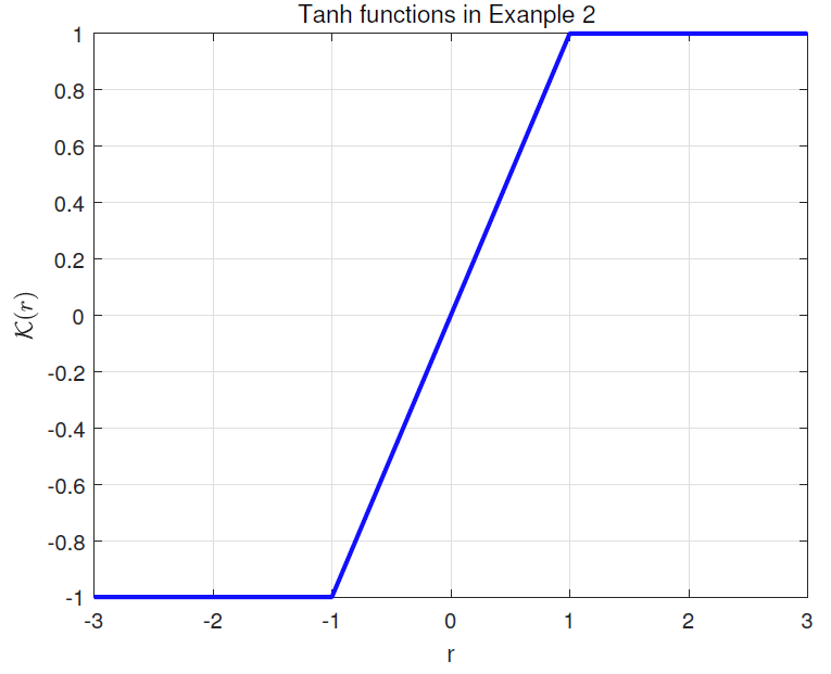
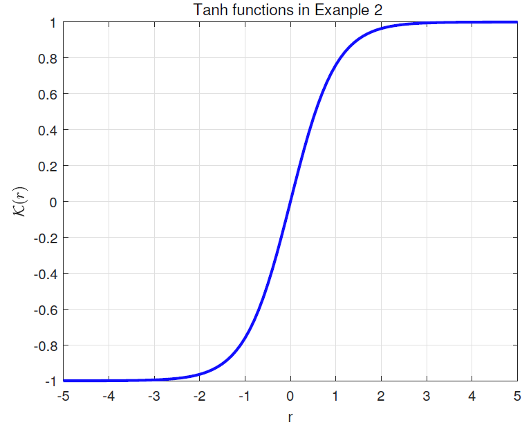
此时激活函数为 $ f(r) = {\rm tanh}(r) $, 几何形状如图1 所示, 且有

此外,有 $\mu _{1}^{*}=\mu _{2}^{*}=0$, $\bar{\delta}_{11}=0.68$, $\bar{\delta}_{22}=0$, $\hat{\rho}_{11}^{s}=0.2$, $\hat{\rho}_{12}^{s}=\hat{\rho}_{21}^{s}=0.15$, $\hat{\rho}_{22}^{s}=0.3$, $\hat{\delta}_{11}^{s}=\hat{\delta}_{22}^{s}=0$, $\hat{\delta}_{12}^{s}=\hat{\delta}_{21}^{s}=0.25$, 验证定理 3.1-定理 3.4 的所需条件可以被满足, 因此根据定理 3.1-定理 3.4 可知 SFCGNNs 具有 $25$ 个平衡点, 其中 $9$ 个平衡点是渐近稳定的, 而其余 $16$ 个平衡点不稳定.

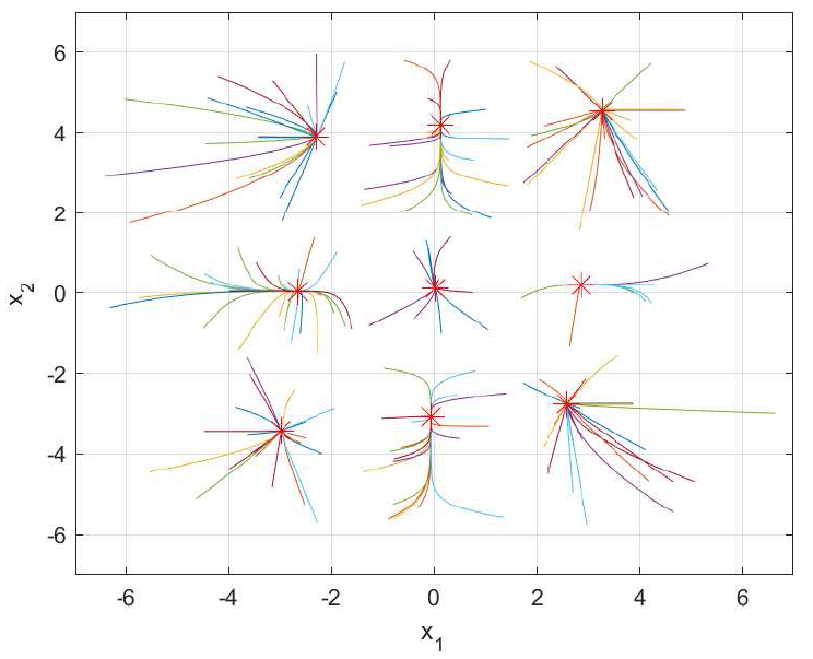
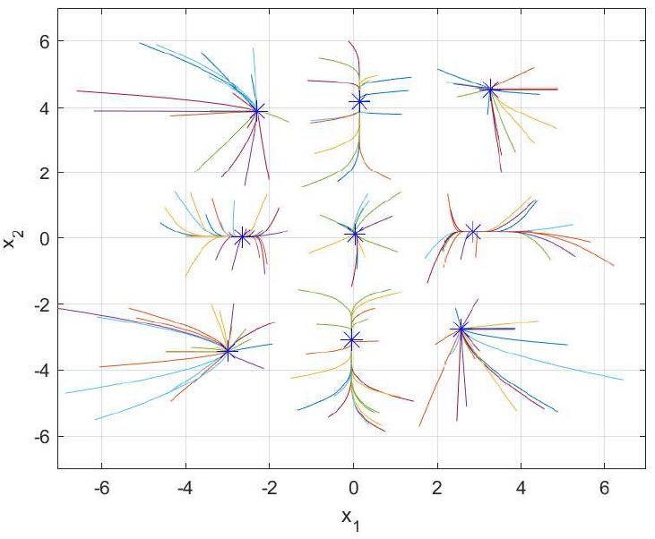
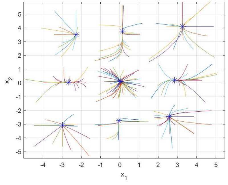
为了验证时变时延对神经网络产生的影响, 考虑 SFCGNNs(4.1)具有条件 $\rho_{11}(x_{1}(t))=\rho_{12}(x_{2}(t))=\rho_{21}(x_{1}(t))=\rho_{22}(x_{2}(t))=0$. 在此条件下,随机选取了 150 个初始值 $x(0) \in [-6, 6] \times [-6, 6]$ 进行数值仿真, 仿真结果如图3 所示, 其中使用红色符号 $*$ 标记稳定的平衡点所在位置. 作为对比, 考虑时变时延为 $t_\tau=(0.5\sin(t)-1)$, $t\ge 0$, 此时时变时延对 SFCGNNs(4.1)产生的影响如 SFCGNNs(4.1)中的参数所示, 选取同样的初始条件, 最后数值仿真结果表示在图4 并使用蓝色符号 $*$ 标记稳定的平衡点所在位置. 仿真结果表明, 时变时延的存在不会影响稳定的平衡点的数量, 这说明本文的推导条件和结果在时延存在的情况下仍然成立.

需要注意的是, 在例 1 中有 $\alpha_2'=\alpha_2''=1$, 此时 Cohen-Grossberg 神经网络就变成了 Hopfield 神经网络, 所以本文的结果同样适用于切换分数阶 Hopfield 神经网络. 而对于切换分数阶递归神经网络, 接下来将给出例 2, 说明在 $\alpha_i'=\alpha_i''=1$ 且 $\mu_i'=\mu_i''=1$ 时, SFCGNNs (1) 的结果同样适用于分数阶递归神经网络.

例 2. 考虑一个二维的 SFCGNNs, 其激活函数如图2 所示,

对于 $t\ge 0$, 其中

根据上述参数, 可以计算出 $\mu_{i}^{*},\bar{\delta}_{ij},\hat{\rho}_{ij}^{s},\hat{\delta}_{ij}^{s}$, 从而确定在 $c_1=c_2=1$ 时, 定理 3.3 的条件对 SFCGNNs 均成立. 我们可以得出结论: SFCGNNs 具有 $ 5\times5=25$ 个平衡点, 其中 $3\times3=9$ 个平衡点是渐近稳定的, 而其余 $16$ 个平衡点是不稳定的. 随机选取 150 个初始条件 $x(0) \in [-5, 5] \times [-5, 5]$ 的仿真图像表示在图5, 其中蓝色符号 $*$ 为稳定的平衡点所在位置. 因此通过上述算例, 可知本论文所推导的的理论成果不仅可用于 Hopfield 神经网络的多稳定分析, 还可用于递归神经网络^[32]的多稳定性分析, 更具有一般性.

在本文中, 研究了具有时变时延的 SFCGNNs 的多重平衡点的稳定性与不稳定性, 得到了确定 SFCGNNs 存在 $ 5^n $ 个平衡点的充分条件, 其中 $ 3^n $ 个平衡点是渐近稳定的, 确定了其余 $ 5^n - 3^n $ 个平衡点不稳定的充分条件. 并且本文所给出的 SFCGNNs 的参数若取特殊值, 如在 $ \alpha_1=\alpha_2=1 $ 时, SFCGNNs (1) 变为切换分数阶 Hopfield 神经网络, 在此条件的基础上再有 $ \mu _1=\mu_2=1 $, SFCGNNs (1) 则是分数阶递归神经网络. 本文推导的理论结果仍然成立. 在未来, 可能会探索具有更强非线性激活函数的 SFCGNNs 的多稳定性.