1 引言
考虑广义互补问题 (Generalized Complementarity Problem, GCP)[1 ] , 即求向量 $x\in\mathbb{R}^{n}$
(1.1) $\begin{equation} F(x)\geq0, G(x)\geq0, \langle F(x),G(x)\rangle=0, \end{equation}$
其中 $F(x)=(F_{1}(x),\cdots,F_{n}(x))^{\text{T}}$ $G(x)=(G_{1}(x),\cdots,G_{n}(x))^{\text{T}}$ . $F_{i}(x)$ $G_{i}(x)$ $i=1,2,\cdots,n$ ) 为 $\mathbb{R}^{n}\rightarrow \mathbb{R}$ $F(x)=Mx+q$ $M\in \mathbb{R}^{n\times n}, q\in\mathbb{R}^{n}), G(x)=x$ [2 ] ; 当 $G(x)=x$ [3 ] ; 当 $G(x)=x-E(x)$ $E(x)$ [4 ] .
GCP (1.1) 的一类重要求解方法是利用一类互补函数, 将其等价转化为非线性方程组, 之后构造价值函数, 通过极小化价值函数并运用相关算法求解该非线性方程组得到GCP (1.1) 的解.
Fischer-Burmeister 函数是一类重要的互补函数[5 ] , 其形式为
(1.2) $\begin{equation} \varphi(a,b)=\sqrt{a^2+b^2}-a-b. \end{equation}$
(1.3) $\begin{equation} \varphi(a,b)=0 \Leftrightarrow a\geq0, b\geq0, ab=0. \end{equation}$
根据 (1.3) 式, 求解 GCP (1.1) 转化为求解非线性方程组
(1.4) $\begin{equation} \Phi(x)=\left(\begin{matrix} \varphi(F_{1}(x),G_{1}(x))\\ \vdots\\ \varphi(F_{n}(x),G_{n}(x)) \end{matrix} \right)=0. \end{equation}$
函数 $\Psi: \mathbb{R}^{n}\rightarrow \mathbb{R}$
(1.5) $\begin{equation} \Psi(x)=\frac{1}{2}\Phi(x)^{\text{T}}\Phi(x)=\frac{1}{2}\|\Phi(x)\|^{2}. \end{equation}$
事实上, 当非线性方程组 (1.4) 的解集非空时, 求解 (1.4) 等价于求解无约束极小化问题
(1.6) $\begin{equation} \underset{x\in \mathbb{R}^{n}}{\text{min}}\Psi(x), \end{equation}$
其中 $\Psi(x)$ $\Psi(x)$
牛顿法是求解非线性方程组的基本迭代方法之一, 其算法构造过程是对非线性方程组 (1.4) 等式左端非线性函数 $\Phi(x)$
另 $\Phi'(x_{k})=V_{k}$ $V_{k}\in\partial\Phi(x_{k})$ $\partial\Phi(x_{k})$ $\Phi(x)$ $x_{k}$ 6 9]. 高斯-牛顿法的迭代格式为
(1.7) $\begin{equation} x_{k+1}=x_{k}+d_{k}^{\text{GN}}, \end{equation}$
其中 $d_{k}^{\text{GN}}=-(V_{k}^{\text{T}}V_{k})^{-1}V_{k}^{\text{T}}\Phi(x_{k})$ $d_{k}^{\text{GN}}$ $d_{k}^{\text{GN}}$
的极小解. 若 $V_{k}$ $d_{k}^{\text{GN}}$ $x_{k+1}=x_{k}+d_{k}^{\text{GN}}$ $V_{k}$ $V_{k}$ $V_{k}^{\text{T}}V_{k}$ $V_{k}$ $V_{k}^{\text{T}}V_{k}$ $V_{k}^{\text{T}}V_{k}+\sigma_{k}I$ $\sigma_{k}>0$ $I$
(1.8) $\begin{equation} x_{k+1}=x_{k}-(V_{k}^{\text{T}}V_{k}+\sigma_{k}I)^{-1}V_{k}^{\text{T}}\Phi(x_{k}), \end{equation}$
(1.9) $\begin{equation} d_{k}=-(V_{k}^{\text{T}}V_{k}+\sigma_{k}I)^{-1}V_{k}^{\text{T}}\Phi(x_{k}). \end{equation}$
(1.8) 式称为 Levenberg-Marquardt 方法, 简称 LM 方法. 该方法也是求解非线性方程组的一类有效方法.
对于 LM 方法求解互补问题等问题的研究, 诸多学者在理论上和算法上取得了较为丰富的研究成果[10 15] . Facchinel 等[10 ] 提出了求解大规模非线性互补问题的非光滑非精确 LM 算法, 在适当的条件下证明了算法的全局收敛性和超线性收敛性; 刘志敏等[11 ] 利用一类广义互补函数, 提出了求解线性互补问题的 LM 算法, 在适当条件下分析了算法的收敛性; 胡雅伶等[12 ] 基于模变换, 提出了求解非线性互补问题的多步自适应 LM 算法, 在一定条件下分析了算法的全局收敛性; Chen 等[14 ] 提出了一类求解非线性方程组的修正的 LM 算法, 并证明了算法的超线性收敛性.
对于 GCP (1.1) 在理论与算法方面的研究上, Du[16 ] 对由一类互补函数构成的非线性方程组进行非光滑重构, 提出了求解 GCP (1.1) 的广义牛顿算法, 在适当的条件下证明了算法的全局收敛性和超线性收敛性; Vivas 等[17 ] 运用一类单参数互补函数和 Armijo 线搜索准则, 提出了求解 GCP (1.1) 的非光滑牛顿算法, 在适当的条件下证明了算法的局部收敛性和 Q-二次收敛性.
另外, 对于 LM 算法的数值性能, LM 参数 $\sigma_{k}$ [18 ] 提出 $\sigma_{k}=\|\Phi(x_{k})\|^{\delta}, \delta\in [1,2]$ [19 ] 提出 $\sigma_{k}=\eta\|\Phi(x_{k})\|+(1-\eta)\|V_{k}^{\text{T}}\Phi(x_{k})\|, \eta\in[0, 1]$ [14 ] 提出 $\sigma_{k}=\eta\|\Phi(x_{k})\|^{\delta}+(1-\eta)\|V_{k}^{\text{T}}\Phi(x_{k})\|^{\delta}, \delta\in [1,2], \eta\in[0, 1]$ . 关于 LM 参数的其他选择, 可参见文献[20 22].
本文构建的 LM 参数为 $\sigma_{k}=\frac{\eta\left\|\Phi(x_{k})\right\|^{\delta}}{1+\eta\|\Phi(x_{k})\|^{\delta}}$ $\delta\in [1,2]$ $\eta>0$ $k$ $\|\Phi(x_{k})\|$ $\|\Phi(x_{k})\|$ $\sigma_{k}$ $\|\Phi(x_{k})\|$ $\sigma_{k}$ $\eta$ $\delta$ $\|\Phi(x_{k})\|$ $\sigma_{k}$
LM 算法在求解线性互补问题、非线性互补问题等问题中有较好的效果[11 ,12 ,23 ,24 ] , 但目前关于 LM 算法求解 GCP (1.1) 的相关研究还较为匮乏. 基于已有文献启发, 本文利用 LM 算法求解 GCP. 结合 Fischer-Burmeister 函数, 将 GCP 等价重构为非光滑非线性方程组, 基于一类自适应修正的 LM 参数和 Armijo 线搜索准则, 提出求解 GCP (1.1) 的一类带有线搜索的自适应修正的 LM 算法. 在适当条件下分析算法的收敛性, 并通过数值实验验证算法的有效性.
本文的后续结构安排如下: 第 2 节陈述本文所需的预备知识; 第 3 节提出求解 GCP (1.1) 的 LM 算法并分析其收敛性; 第 4 节通过数值实验验证所提出算法的有效性; 第 5 节给出本文的结论.
本文的符号说明如下: $\mathbb{R}$ $\mathbb{R}^{n}$ $n$ $\mathbb{R}^{m\times n}$ $m\times n$ $\|\cdot\|$ $I$ $\nabla F(x)=F'(x)^{\text{T}}$ $F$ $x$ $\emptyset$ $\mathbb{M}=\{1,2,\cdots,n\}$ $\text{diag}\{x_{i}:i\in\mathbb{M}\}$ $i$ $x_{i}$ $e_{n}=(1,1,\cdots,1)^{\text{T}}\in\mathbb{R}^{n}$ . $\text{rank} (A)$ $A$ $a=\textit{O}(b)$ $\text{lim} \underset{b\rightarrow0}{\text{sup}}\frac{a}{b}<+\infty$ . $\text{tridiag}(a,b,c)$ $a$ $b$ $c$ $\text{tridiag}(A,B,C)$ $A$ $B$ $C$
2 预备知识
定义2.1 [25 ] 函数 $H:\mathbb{R}^{n}\rightarrow \mathbb{R}^{n}$ $D_{H}$ $H$ $\forall x\in \mathbb{R}^{n}$ $H$ $x$
定义2.2 [26 ] 函数 $H$
即 $\partial H(x)$ $\partial_{B}H(x)$
定义2.3 [27 ] 如果矩阵 $A\in\mathbb{R}^{n\times n}$ $A$ $P_{0}$ - 矩阵.
定义2.4 [18 ] 设集合 $\mathbb{N}\subset\mathbb{R}^{n}$ $\mathbb{N}\cap \mathbb{X^{*}}\neq\emptyset$ $\mathbb{X^{*}}$ $\gamma$
(2.1) $\begin{equation} \|\Phi(x)\|\geq \gamma\text{dist}(x, \mathbb{X^{*}}), \forall x\in\mathbb{N}, \end{equation}$
则称 $\|\Phi(x)\|$ $\Phi(x)=0$ $\mathbb{N}$ $\text{dist}(x, \mathbb{X^{*}})=\underset{y\in \mathbb{X^{*}}}{\text{inf}}\|y-x\|$ .
引理2.1 [5 ,28 ] $\varphi(a,b)$ $\varphi(a,b)$
接下来给出 $\Phi(x)$ $\Phi_{i}(x)$
命题2.1 设 $\Phi_{i}(x)=\varphi(F_{i}(x),G_{i}(x))$ $i\in\{1,2,\cdots,n\}$ $(F_{i}(x),G_{i}(x))\neq(0,0)$ $\Phi_{i}(x)$ $x$
(2.2) $\begin{equation} \nabla \Phi_{i}(x)=\text{diag}(a_{i}(x))\nabla F_{i}(x)+\text{diag}(b_{i}(x))\nabla G_{i}(x), \end{equation}$
(2.3) $\begin{equation} a_{i}(x)=\frac{F_{i}(x)}{\sqrt{F_{i}(x)^2+G_{i}(x)^2}}-1, \end{equation}$
(2.4) $\begin{equation} b_{i}(x)=\frac{G_{i}(x)}{\sqrt{F_{i}(x)^2+G_{i}(x)^2}}-1. \end{equation}$
命题2.2 定义集合 $K=\left\{x\in\mathbb{R}^{n}|(F_{i}(x))^{2}+(G_{i}(x))^{2}>0, i=1,2,\cdots,n\right\}$ $D_{a}(x)=\text{diag}\left(a_{1}(x),\cdots, a_{n}(x)\right)$ $D_{b}(x)=\text{diag}(b_{1}(x),\cdots, b_{n}(x))$ . $a_{i}(x)$ $b_{i}(x)$
+++2. 当 $x\notin K$ $V(x)\in\partial\Phi(x)$
(2.5) $\begin{equation} V(x)=D_{a}(x)\nabla F(x)+D_{b}(x)\nabla G(x). \end{equation}$
证 证明过程类似文献 [命题 2]、[命题 3], 故在此省略.
下面的命题给出了价值函数 $\Psi(x)$ $\Phi(x)$
命题2.3 连续可微的函数 $\Psi(x)$ $V(x)\in\partial\Phi(x)$ $\nabla\Psi(x)=V(x)^{\text{T}}\Phi(x)$ .
证 证明过程类似文献[28 ,命题 3.4], 故在此省略.
3 算法及收敛性分析
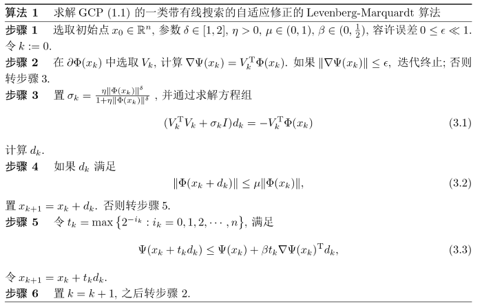
本节提出求解 GCP (1.1) 的一类带有线搜索的自适应修正的 Levenberg-Marquardt 算法, 即算法1, 并分析算法的收敛性. 该算法的基本思想是通过极小化价值函数 $\Psi(x)$ $\Phi(x)=0$ .
证 由算法 1 的步骤 2 知, 如果 $\|\nabla\Psi(x_{k})\|\leq\epsilon$ $\nabla\Psi(x_{k})>0$ . 由于 $\nabla\Psi(x_{k})=V_{k}^{\text{T}}\Phi(x_{k})\neq0$ $\Phi(x_{k})\neq0$ . 故由 $\sigma_{k}$ $\sigma_{k}$ $V_{k}^{\text{T}}V_{k}+\sigma_{k}I$ $I$ $V_{k}^{\text{T}}V_{k}$ $V_{k}^{\text{T}}V_{k}+\sigma_{k}I$ $d_{k}$
(3.4) $\begin{equation} \nabla\Psi(x_{k})^{\text{T}}d_{k}=-\nabla\Psi(x_{k})^{\text{T}}(V_{k}^{\text{T}}V_{k}+\sigma_{k}I)^{-1}\nabla\Psi(x_{k})<0, \end{equation}$
这意味着 $d_{k}$ $\Psi(x)$ $x_{k}$
在上式中令 $i\rightarrow\infty$ $\Psi(x)$ $\nabla\Psi(x_{k})^{\text{T}}d_{k}\geq\beta\nabla\Psi(x_{k})^{\text{T}}d_{k}$ . 此结合 $\beta\in(0,\frac{1}{2})$ $\nabla\Psi(x_{k})^{\text{T}}d_{k}\geq0$
当 GCP (1.1) 无解时, $\Psi(x)$ $x^{*}$ $\Psi(x^{*})>0$ . 另外, 值得关注的一个情形是 $\Psi(x)$ $\Psi(x)$
引理3.1 [1 ] 如果 GCP (1.1) 的解集是非空的, 则 $x^{*}\in\mathbb{R}^{n}$ $\Psi(x^{*})=0$ .
引理3.2 [1 ] 假设函数 $F,G$ $x^{*}$ $\Psi(x)$ $G'(x^{*})$ $F'(x^{*})G'(x^{*})^{-1}$ $P_{0}$ - 矩阵, 那么 $x^{*}$
根据定义 2.4, 如果 $\overline{x}\in\mathbb{X}^{*}$ $V(\overline{x})$ $\overline{x}$ $\|\Phi(x)\|$ $\overline{x}$ 29 ]. 因此局部误差界条件要比非奇异性条件弱.
下面分析算法 1 的收敛性, 在证明收敛性的结论之前, 需要以下假设和结论.
假设3.1 $\Phi(x)$ $V(x)$ $\overline{x}\in\mathbb{X}^{*}$ $L_{1},L_{2}$ $b<0.5$
(3.5) $\begin{equation} \|V(y)-V(x)\|\leq2L_{1}\|y-x\|, \end{equation}$
(3.6) $\begin{equation} \|\Phi(y)-\Phi(x)\|\leq L_{2}\|y-x\|, \end{equation}$
(3.7) $\begin{equation} \|\Phi(y)-\Phi(x)-V(x)(y-x)\|\leq L_{1}\|y-x\|^{2} \end{equation}$
在 $\forall x,y\in\mathbb{N} (\overline{x},2b)=\left\{x | \|x-\overline{x}\|\leq2b\right\}$
假设3.2 $\|\Phi(x)\|$ $\Phi(x)=0$ $\mathbb{N}(\overline{x},2b)$ $\gamma_{1}>0$
(3.8) $\begin{equation} \|\Phi(x)\|\geq\gamma_{1}\text{dist}(x,\mathbb{X^{*}}), \forall x\in\mathbb{N}(\overline{x},2b). \end{equation}$
其中 $\delta\in [1,2]$ $\eta>0$ $\overline{x}_{k}\in\mathbb{X^{*}}$ $\|x_{k}-\overline{x}_{k}\|=\text{dist}(x_{k},\mathbb{X}^{*})$
引理3.3 如果假设 3.1 和假设 3.2 成立, $x_{k}\in \mathbb{N}(\overline{x},b)$ $k$
证 对于任意充分大的 $k$
下面从两方面考虑: 如果 $\|\Phi(x_{k})\|\leq1$ $\|\Phi(x_{k})\|^{\delta}\leq1$ $1+\|\Phi(x_{k})\|^{\delta}\leq2$ . 由 (3.8) 式得
如果 $\|\Phi(x_{k})\|\geq1$ $\|\Phi(x_{k})\|^{\delta}\geq1$ $1+\|\Phi(x_{k})\|^{\delta}\leq2\|\Phi(x_{k})\|^{\delta}$
综上分析, $\rho_{k}\leq\sigma_{k}\leq \eta L_{2}^{\delta}\|x_{k}-\overline{x}_{k}\|^{\delta}$ $\rho_{k}=\min\left\{\frac{\eta}{1+\eta}, \frac{\eta}{2}\gamma_{1}^{\delta}\|x_{k}-\overline{x}_{k}\|^{\delta}\right\}$ .
引理3.4 如果假设 3.1 成立, $x_{k}\in\mathbb{N}(\overline{x},b)$ $\gamma_{2}>0$
(3.9) $\begin{equation} \|d_{k}\|\leq \gamma_{2}\text{dist}(x_{k},\mathbb{X}^{*}). \end{equation}$
证 由 $x_{k}\in\mathbb{N}(\overline{x},b)$
即 $\overline{x}_{k}\in\mathbb{N}(\overline{x},2b)$ .
由 (1.9) 式知, $d_{k}$ $\phi_{k}(d)$
因此, 当 $\overline{x}_{k}\in\mathbb{N}(\overline{x},2b)$ $b<0.5$
即 $\|d_{k}\|\leq\gamma_{2}\text{dist}(x_{k},\mathbb{X}^{*})$ $\gamma_{2}=\sqrt{\eta^{-1}L_{1}^{2}\gamma_{1}^{-\delta}+\gamma_{1}^{-\delta}L_{1}^{2}L_{2}^{\delta}+1}$ .
引理3.5 如果假设 3.1 和假设 3.2 成立, $x_{k+1}, x_{k}\in \mathbb{N}(\overline{x},b)$ $\gamma_{3}>0$
(3.10) $\begin{equation} \text{dist}(x_{k}+d_{k},\mathbb{X}^{*})\leq\gamma_{3}\text{dist}(x_{k},\mathbb{X}^{*})^{\frac{2+\delta}{2}}. \end{equation}$
由引理 3.3 知, $\sigma_{k}\leq \eta L_{2}^{\delta}\|x_{k}-\overline{x}_{k}\|^{\delta}$
假设 $\|x_{k}-\overline{x}_{k}\|<1$
其中 $\gamma_{3}=\left(\sqrt{L_{1}^{2}+\eta L_{2}^{\delta}}+L_{1}\gamma_{2}^{2}\right)/\gamma_{1}$ .
接下来运用奇异值分解理论分析 LM 算法的收敛性. 不失一般性, 假设 $\{x_{k}\}$ $\mathbb{X}^{^{*}}$ $\overline{x}$ $\overline{x}\in\mathbb{X}^{*}$ 30 ], 如果 $\|\Phi(x)\|$ $\nu>0$
假设对所有的 $x\in\mathbb{N}(\overline{x},2b)\cap\mathbb{X}^{*}$ $\text{rank}(V(x))=r$ .
假定 $V(\overline{x}_{k})$
其中 $\overline{\Sigma}_{k,1}=\text{diag}(\overline{\theta}_{k,1},\overline{\theta}_{k,2},\cdots,\overline{\theta}_{k,r})$ $\overline{\theta}_{k,1}\geq \overline{\theta}_{k,2}\geq\cdots\geq\overline{\theta}_{k,r}>0$ . 相应地, $V(x_{k})$
(3.11) $\begin{align*} V(x_{k})&=U_{k}\Sigma_{k}J_{k}^{\text{T}}\nonumber\\ &=\left(U_{k,1},U_{k,2},U_{k,3}\right)\left(\begin{matrix}\Sigma_{k,1}&0&0\nonumber\\ 0&\Sigma_{k,2}&0\\ 0&0&0 \end{matrix} \right) \left(\begin{matrix} J_{k,1}^{\text{T}}\\ J_{k,2}^{\text{T}}\\ J_{k,3}^{\text{T}} \end{matrix} \right)\\ &=U_{k,1}\Sigma_{k,1}J_{k,1}^{\text{T}}+U_{k,2}\Sigma_{k,2}J_{k,2}^{\text{T}}, \end{align*}$
其中 $\Sigma_{k,1}=\text{diag}(\theta_{k,1},\theta_{k,2},\cdots,\theta_{k,r})$ $\Sigma_{k,2}=\text{diag}(\theta_{k,r+1},\theta_{k,r+2},\cdots,\theta_{k,r+s})$ $\theta_{k,1}\geq\theta_{k,2}\geq\cdots\geq\theta_{k,r}>0$ $\theta_{k,r+1}\geq\theta_{k,r+2}\geq\cdots\geq\theta_{k,r+s}>0$ . 为方便分析, 省略 $\Sigma_{k,i} (i=1,2)$ $U_{k,i}$ $J_{k,i} (i=1,2,3)$ $k$
(3.12) $\begin{equation} V_{k}=U\Sigma J^{\text{T}}=U_{1}\Sigma_{1}J_{1}^{\text{T}}+U_{2}\Sigma_{2}J_{2}^{\text{T}}. \end{equation}$
引理3.6 如果假设 3.1 成立, $x_{k}\in\mathbb{N}(\overline{x},b)$
1. $\|U_{1}U_{1}^{\text{T}}\Phi(x_{k})\|\leq L_{2}\|x_{k}-\overline{x}_{k}\|$
2. $\|U_{2}U_{2}^{\text{T}}\Phi(x_{k})\|\leq4L_{1}\|x_{k}-\overline{x}_{k}\|^{2}$
3. $\|U_{3}U_{3}^{\text{T}}\Phi(x_{k})\|\leq L_{1}\|x_{k}-\overline{x}_{k}\|^{2}$ .
证 由 (3.6) 式易得结论 1. 根据矩阵扰动理论[31 ] 和 (3.5) 式, 得到
(3.13) $\begin{equation} \|\Sigma_{1}-\overline{\Sigma}_{1}\|\leq 2L_{1}\|x_{k}-\overline{x}_{k}\|, \|\Sigma_{2}\|\leq 2L_{1}\|x_{k}-\overline{x}_{k}\|. \end{equation}$
令 $V_{k}^{+}$ $V_{k}$ $q_{k}=-V_{k}^{+}\Phi(x_{k})$ $q_{k}$ $\text{min}\|\Phi(x_{k})+V_{k}q\|$
令 $\overline{V}_{k}=U_{1}\Sigma_{1}J_{1}^{\text{T}}$ $\overline{q}_{k}=-\overline{V}_{k}^{+}\Phi(x_{k})$ . 因为 $\overline{q}_{k}$ $\text{min}\|\Phi(x_{k})+\overline{V}_{k}\overline{q}\|$
定理3.2 如果假设 3.1 和假设 3.2 成立, 则由 (1.8) 式生成的迭代序列 $\{x_{k}\}$ $\overline{x}\in\mathbb{X}^{*}$ .
(3.14) $\begin{align*} \Phi(x_{k})+V_{k}d_{k}&=\Phi(x_{k})-U_{1}\Sigma_{1}(\Sigma_{1}^{2}+\sigma_{k}I)^{-1}\Sigma_{1}U_{1}^{\text{T}}\Phi(x_{k})- U_{2}\Sigma_{2}(\Sigma_{2}^{2}+\sigma_{k}I)^{-1}\Sigma_{2}U_{2}^{\text{T}}\Phi(x_{k}) \nonumber\\ &=\sigma_{k}U_{1}(\Sigma_{1}^{2}+\sigma_{k}I)^{-1}U_{1}^{\text{T}}\Phi(x_{k})+ \sigma_{k}U_{2}(\Sigma_{2}^{2}+\sigma_{k}I)^{-1}U_{2}^{\text{T}}\Phi(x_{k})+U_{3}U_{3}^{\text{T}}\Phi(x_{k}). \end{align*}$
不失一般性, 假设 $\|x_{k}-\overline{x}_{k}\|\leq\overline{\theta}_{r}/(4L_{1})$ $k$
由上面两个不等式、引理 3.3、引理 3.6 和 (3.14) 式得
令 $\gamma_{4}=\left(4\eta L_{2}^{1+\delta}/\overline{\theta}_{r}^{2}\right)+5L_{1}$ $k$
由引理 3.4 得$\|d_{k+1}\|=\textit{O}\left(\|d_{k}\|^{2}\right),$ $\{x_{k}\}$ $\overline{x}\in\mathbb{X}^{*}$
引理3.7 [18 ] 如果梯度 $\nabla\Psi(x)=V(x)^{\text{T}}\Phi(x)$ $t_{k}$ $\xi_{1},\xi_{2}$
(3.15) $\begin{equation} \Psi(x_{k+1})\leq\Psi(x_{k})-\xi_{1}\xi_{2}\frac{(\nabla\Psi(x_{k})^{\text{T}}d_{k})^{2}}{\|d_{k}\|^{2}}. \end{equation}$
定理3.3 设 $\{x_{k}\}$ $\sigma_{k}=\frac{\eta\|\Phi(x_{k})\|^{\delta}}{1+\eta\|\Phi(x_{k})\|^{\delta}}$ $\eta>0$ $\delta\in [1,2]$ $\{x_{k}\}$ $\overline{x}$ $\Psi(x)$ $\{x_{k}\}$ $\overline{x}\in\mathbb{X}^{*}$ .
证 首先证明第一部分结论. 由 (3.15) 式知, 非负序列 $\left\{\|\Phi(x_{k})\|\right\}$ $\underset{k\rightarrow\infty}{\text{lim}}\|\Phi(x_{k})\|:=\tau$ $\tau=0$ $\Phi(x)$ $\Phi(\overline{x})=0$ $\tau>0$ $k$ $k$
(3.16) $\begin{equation} \underset{k\rightarrow\infty}{\text{lim}}\frac{\left(\nabla\Psi(x_{k})^{\text{T}}d_{k}\right)^{2}}{\|d_{k}\|^{2}}=0. \end{equation}$
由上式和 (3.16) 式得$\underset{k\rightarrow\infty}{\text{lim}}\|d_{k}\|=0.$ $V(x)$ $\nabla\Psi(\overline{x})=0$ . 第一部分证毕.
接下来证明第二部分结论. 这一部分只需证明对于任意充分大的 $k$ $\overline{x}\in\mathbb{X}^{*}$ $\overline{k}$ $x_{\overline{k}}\in\mathbb{N}(\overline{x},r)$
由 $x_{\overline{k}}\in\mathbb{N}(\overline{x},r)$ $\forall k\geq \overline{k}$ $x_{\overline{k}}\in\mathbb{N}(\overline{x},b)$ . 由引理 3.3、(3.9) 式和 (3.10) 式得
即对于 $\forall k\geq\overline{k}$ $\|\Phi(x_{k+1})\|\leq\mu\|\Phi(x_{k})\|.$ $\{x_{k}\}$ $k$ $t_{k}=1$ . 二次收敛性得证.
4 数值实验
本节通过数值实验验证算法 1 的性能. 数值实验在 Windows10 操作系统, AMD 锐龙 7 6800H 处理器 3.20 GHz, 内存 16.0 GB 配置的 64 位操作系统的个人计算机上进行, 使用 MATLAB R2018a 软件进行程序设计与实现. 实验中与文献[14 ,18 ]中的两类 LM 算法进行性能对比.
算法 1 (NLLM) 中选取参数 $\eta=0.5$ $\delta=1$ $\beta=10^{-4}$ $\mu=0.9$ $\sigma_{k}=\frac{\eta\|\Phi(x_{k})\|^{\delta}}{1+\eta\|\Phi(x_{k})\|^{\delta}}$ $\delta\in [1,2]$ $\eta>0$ 18 ]中的带有线搜索的 LM 算法 (NLM) 中选取参数 $\delta=1$ $\sigma_{k}=\|\Phi(x_{k})\|^{\delta}$ $\delta\in [1,2]$ 14 ]中带有线搜索的改进的 LM 算法 (MLM) 中选取参数 $\eta=0.5, \delta=1$ $\sigma_{k}=\eta\|\Phi(x_{k})\|^{\delta}+(1-\eta)\|V_{k}^{\text{T}}\Phi(x_{k})\|^{\delta}$ $\eta\in[0, 1]$ $\delta\in [1,2]$ . 对于三种算法, 停止准则均为 $\|\nabla\Psi(x_{k})\|\leq10^{-8}$ $n$ $\|\nabla\Psi(x_{k})\|$ $\|\nabla\Psi(x_{k})\|$
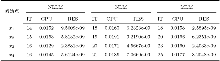
例 4.1 [16 ] 考虑 GCP (1.1), 其中 $F,G:\mathbb{R}^{2}\rightarrow \mathbb{R}^{2}$
该问题的解为 $x^{*}_{1}=(0,0)^{\text{T}}$ . 选取初始点 $x_{1}=(3,3)^{\text{T}}, x_{2}=(5,5)^{\text{T}}, x_{3}=(10,1)^{\text{T}}, x_{4}=(10,10)^{\text{T}}$ . 求解例 4.1 的数值实验结果如表1 所示.
例 4.2 [32 ] 考虑 GCP (1.1), 其中 $F,G:\mathbb{R}^{2}\rightarrow \mathbb{R}^{2}$
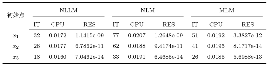
该问题的解是 $x^{*}_{1}=(10,5)^{\text{T}}$ $x^{*}_{2}=(20,15)^{\text{T}}$ . 选取初始点 $x_{1}=(0,10)^{\text{T}}$ $x_{2}=(18,0)^{\text{T}}$ $x_{3}=(11,0)^{\text{T}}$ . 求解例 4.2 的数值实验结果如表2 所示.
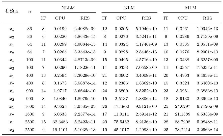
例 4.3 [33 ] 考虑 GCP (1.1), 其中 $F,G:\mathbb{R}^{n}\rightarrow \mathbb{R}^{n}$ $F(x)=Ax+q+\theta(x), G(x)=x-\gamma(x),$ $A\in \mathbb{R}^{n\times n}$ $q=(-1,1,\cdots,(-1)^{n})^{\text{T}}\in \mathbb{R}^{n}$ $\theta(x)=(x_{1}^{2},x_{2}^{2},\cdots,x_{n}^{2})^{\text{T}}\in\mathbb{R}^{n}$ $\gamma(x)=(x_{1}^{3},x_{2}^{3},\cdots,x_{n}^{3})^{\text{T}}\in\mathbb{R}^{n}$
该问题的解是 $x^{*}_{1}=e_{n}$ . 选取初始点 $x_{1}=(1,0.6,1,0.6,\cdots)^{\text{T}}$ $x_{2}=(0,0,\cdots)^{\text{T}}$ . 选取不同维数的矩阵进行数值实验, 求解例 4.3 的数值实验结果如表3 所示.
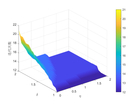
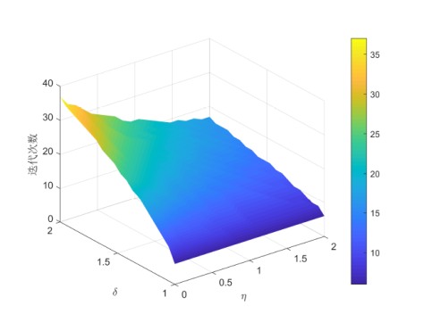
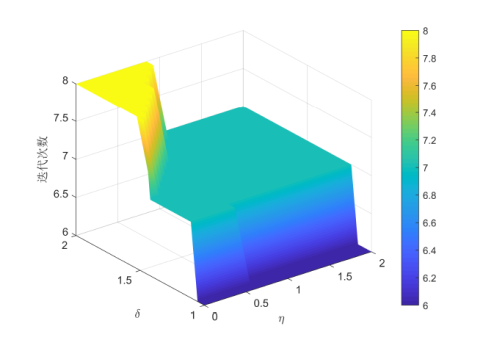
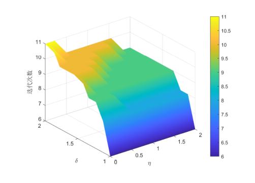
下面列出 $\eta$ $\delta$ $\eta\in[10^{-5},2]$ $\delta\in [1,2]$ . 对于例 4.1, 以选取初始点 $(3,3)^{\text{T}}$ $(11,0)^{\text{T}}$ $\eta$ $\delta$ 图1 、图2 所示. 对于例 4.3, 以矩阵维数分别选取 $n=100$ $2500$ $(0,0,\cdots)^{\text{T}}$ $\eta$ $\delta$ 图3 、图4 所示.
图1
图1
$\eta$ $\delta$
图2
图2
$\eta$ $\delta$
图3
图3
$\eta$ $\delta$ $n=100$ )
图4
图4
$\eta$ $\delta$ $n=2500$ )
从图1 、图2 中可以看出, 当 $\eta$ $\delta$ $\eta$ $\delta$ $\eta$ $\delta$ 图3 、图4 中可以看出, 无论 $\eta$ $\delta$
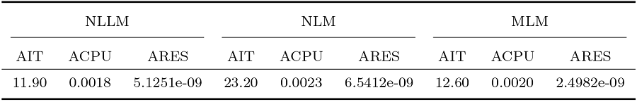
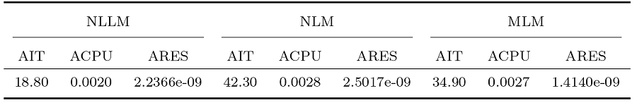
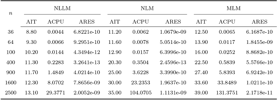
针对 NLLM 算法与 NLM、MLM 算法, 选取初始点为 $x_{0}=\text{rand}(n,1)$ $n$ 表4 -6 所示.
在每一组数值实验中, 针对不同的问题选择不同的初始点对算法进行测试.通过表1 -表6 的数值实验结果可以看出, NLLM 算法都能收敛到对应问题的解.NLLM 算法在IT、AIT、CPU、ACPU 等方面优于NLM、MLM 算法, 这表明NLLM 算法具有良好的性能.
5 结论
基于 Fischer-Burmeister 函数, 自适应修正的 LM 参数和 Armijo 线搜索准则, 本文提出了求解广义互补问题的一类带有线搜索的自适应修正的 Levenberg-Marquardt 算法. 在适当的条件下证明了该算法的二次收敛性. 数值实验结果验证了本文提出的算法是可行且高效的.
参考文献
View Option
[1]
Kanzow C Fukushima M . Equivalence of the generalized complementarity problem to differentiable unconstrained minimization
J Optim Theory Appl , 1996 , 90 581 -603
[本文引用: 3]
[2]
Bai Z Z . Modulus-based matrix splitting iteration methods for linear complementarity problems
Numer Linear Algebra Appl , 2010 , 17 6 ): 917 -933
[本文引用: 1]
[3]
Noor M A . On the nonlinear complementarity problem
J Math Anal Appl , 1987 , 1.3 2 ): 455 -460
[本文引用: 1]
[4]
Pang J S . On the convergence of a basic iterative method for the implicit complementarity problem
J Optim Theory Appl , 1982 , 37 149 -162
[本文引用: 1]
[5]
Fischer A . A special Newton-type optimization method
Optimization , 1992 , 24 3/4 ): 269 -284
[本文引用: 2]
[6]
迟晓妮 , 曾荣 , 刘三阳 , 等 . 对称锥权互补问题的正则化非单调非精确光滑牛顿法
数学物理学报 , 2021 , 41A 2 ): 507 -522
[本文引用: 1]
Chi X N Zeng R Liu S Y , et al . A regularized nonmonotone inexact smoothing Newton algorithm for weighted symmetric cone complementarity problems
Acta Math Sci , 2021 , 41A 2 ): 507 -522
[本文引用: 1]
[7]
张运胜 , 高雷阜 . 对称锥互补问题的一种非精确光滑牛顿算法
数学物理学报 , 2015 , 35A 4 ): 824 -832
Zhang Y S Gao L F . A smoothing inexact Newton method for symmetric cone complementarity problems
Acta Math Sci , 2015 , 35A 4 ): 824 -832
[8]
Mittal G Giri A K . Convergence rates for iteratively regularized Gauss-Newton method subject to stability constraints
J Comput Appl Math , 2022 , 4.0 113744
[9]
Tang J Y Zhou J C . A modified damped Gauss-Newton method for non-monotone weighted linear complementarity problems
Optim Methods Softw , 2022 , 37 3 ): 1145 -1164
[本文引用: 1]
[10]
Facchinei F Kanzow C . A nonsmooth inexact Newton method for the solution of large-scale nonlinear complementarity problems
Math Program , 1997 , 76 493 -512
[本文引用: 2]
[11]
刘志敏 , 杜守强 , 王瑞莹 . 求解线性互补问题的 Levenberg-Marquardt 型算法
应用数学学报 , 2018 , 41 3 ): 403 -419
DOI:10.12387/C2018031
[本文引用: 2]
In this paper, we consider the method for solving linear complementarity problems. By a kind of generalized complementarity function, we transform the linear complementarity problems into the nonlinear equations and use the Levenberg-Marquardt type methods to solve it. Under mild conditions, we give the convergence analysis of the given methods. Finally, the numerical results indicate the efficiency of the given methods.
Liu Z M Du S Q Wang R Y . Levenberg-Marquardt type method for solving linear complementarity problems
Acta Math Appl Sin , 2018 , 41 3 ): 403 -419
DOI:10.12387/C2018031
[本文引用: 2]
In this paper, we consider the method for solving linear complementarity problems. By a kind of generalized complementarity function, we transform the linear complementarity problems into the nonlinear equations and use the Levenberg-Marquardt type methods to solve it. Under mild conditions, we give the convergence analysis of the given methods. Finally, the numerical results indicate the efficiency of the given methods.
[12]
胡雅伶 , 彭拯 , 章旭 , 等 . 一种求解非线性互补问题的多步自适应 Levenberg-Marquardt 算法
计算数学 , 2021 , 43 3 ): 322 -336
DOI:10.12286/jssx.j2019-0615
[本文引用: 2]
A modulus-based manipulation is adopted to transform the nonlinear complementarity problem to a non-smooth system. Then, an adaptive multi-step Levenberg-Marquardt method is generalized to solve the resulting non-smooth system, then obtains a solution of the original problem. Under some suitable conditions, the global convergence of the proposed method is established. Some preliminary numerical experiments show that, compared to the PSA-LMM, the proposed method is more effective.
Hu Y L Peng Z Zhang X , et al . An adaptive multi-step Levenberg-Marquardt method for nonlinear complementarity problem
Math Numer Sin , 2021 , 43 3 ): 322 -336
DOI:10.12286/jssx.j2019-0615
[本文引用: 2]
A modulus-based manipulation is adopted to transform the nonlinear complementarity problem to a non-smooth system. Then, an adaptive multi-step Levenberg-Marquardt method is generalized to solve the resulting non-smooth system, then obtains a solution of the original problem. Under some suitable conditions, the global convergence of the proposed method is established. Some preliminary numerical experiments show that, compared to the PSA-LMM, the proposed method is more effective.
[13]
Lera G Pinzolas M . Neighborhood based Levenberg-Marquardt algorithm for neural network training
IEEE Trans Neural Netw , 2002 , 13 5 ): 1200 -1203
[14]
Chen L Ma Y F . A modified Levenberg-Marquardt method for solving system of nonlinear equations
J Appl Math Comput , 2023 , 69 2019 -2040
[本文引用: 4]
[15]
晋慧慧 , 袁柳洋 , 万仲平 . 一种新的非单调修正 Levenberg-Marquardt 算法
应用数学学报 , 2024 , 47 5 ): 799 -810
DOI:10.20142/j.cnki.amas.202401016
[本文引用: 1]
In this paper, a new nonmonotone modified L-M algorithm for solving nonlinear equations is proposed by combining the nonmonotone line search technique with the modified Levenberg-Marquardt algorithm (L-M algorithm). In each iteration of the new algorithm, a modified step is introduced, and the gradient norm of the value function is used to update the L-M parameters. If the trial step is not accepted, the nonmonotone line search technique is used to obtain the new iteration point. Under certain assumptions, the global convergence and local convergence of the algorithm are proved. Numerical experiment results show that the algorithm is feasible and effective.
Jin H H Yuan L Y Wan Z P . A new nonmonotone modified Levenberg-Marquardt algorithm
Acta Math Appl Sin , 2024 , 47 5 ): 799 -810
DOI:10.20142/j.cnki.amas.202401016
[本文引用: 1]
In this paper, a new nonmonotone modified L-M algorithm for solving nonlinear equations is proposed by combining the nonmonotone line search technique with the modified Levenberg-Marquardt algorithm (L-M algorithm). In each iteration of the new algorithm, a modified step is introduced, and the gradient norm of the value function is used to update the L-M parameters. If the trial step is not accepted, the nonmonotone line search technique is used to obtain the new iteration point. Under certain assumptions, the global convergence and local convergence of the algorithm are proved. Numerical experiment results show that the algorithm is feasible and effective.
[16]
Du S Q . Generalized Newton method for a kind of complementarity problem
Abstr Appl Anal , 2014 , 20.4 (1 ): 745981
[本文引用: 2]
[17]
Vivas H Pérez R Arias C A . A nonsmooth Newton method for solving the generalized complementarity problem
Numer Algorithms , 2024 , 95 551 -574
[本文引用: 1]
[18]
Fan J Y Yuan Y X . On the quadratic convergence of the Levenberg-Marquardt method without nonsingularity assumption
Computing , 2005 , 74 23 -39
[本文引用: 5]
[19]
Ma C F Jiang L H . Some research on Levenberg-Marquardt method for the nonlinear equations
Appl Math Comput , 2007 , 1.4 2 ): 1032 -1040
[本文引用: 1]
[20]
Fan J Y Pan J Y . A note on the Levenberg-Marquardt parameter
Appl Math Comput , 2009 , 2.7 2 ): 351 -359
[本文引用: 1]
[21]
Amini K Rostami F Caristi G . An efficient Levenberg-Marquardt method with a new LM parameter for systems of nonlinear equations
Optimization , 2018 , 67 5 ): 637 -650
[22]
Huang B H Ma C F . A Shamanskii-like self-adaptive Levenberg-Marquardt method for nonlinear equations
Comput Math Appl , 2019 , 77 2 ): 357 -373
[本文引用: 1]
[23]
Tang J Y Zhou J C . Quadratic convergence analysis of a nonmonotone Levenberg-Marquardt type method for the weighted nonlinear complementarity problem
Comput Optim Appl , 2021 , 80 213 -244
[本文引用: 1]
[24]
Liu X J Liu S Y . A smoothing Levenberg-Marquardt method for the complementarity problem over symmetric cone
Appl Math , 2022 , 67 49 -64
[本文引用: 1]
[25]
Lopes V L R Martínez J M Pérez R . On the local convergence of quasi-Newton methods for nonlinear complementarity problems
Appl Numer Math , 1999 , 30 1 ): 3 -22
[本文引用: 1]
[26]
Yang Y F Qi L Q . Smoothing trust region methods for nonlinear complementarity problems with $P_{0}$ - functions
Ann Oper Res , 2005 , 1.3 99 -117
[本文引用: 1]
[27]
Jana R Dutta A Das A K . More on hidden $Z$ - matrices and linear complementarity problem
Linear Multilinear Algebra , 2021 , 69 6 ): 1151 -1160
[本文引用: 1]
[28]
Facchinei F Soares J . A new merit function for nonlinear complementarity problems and a related algorithm
SIAM J Optim , 1997 , 7 1 ): 225 -247
[本文引用: 2]
[29]
Yamashita N Fukushima M . On the rate of convergence of the Levenberg-Marquardt method
Computing , 2001 , 15 239 -249
[本文引用: 1]
[30]
Behling R Iusem A . The effect of calmness on the solution set of systems of nonlinear equations
Math Program , 2013 , 1.7 155 -165
[本文引用: 1]
[31]
Stewart G W Sun J G . Matrix Perturbation Theory . Boston : Academic Press , 1990
[本文引用: 1]
[32]
Outrata J V Zowe J . A Newton method for a class of quasi-variational inequalities
Comput Optim Appl , 1995 , 4 5 -21
[本文引用: 1]
[33]
Wu S L Guo P . Modulus-based matrix splitting algorithms for the quasi-complementarity problems
Appl Numer Math , 2018 , 1.2 127 -137
[本文引用: 1]
Equivalence of the generalized complementarity problem to differentiable unconstrained minimization
3
1996
... 考虑广义互补问题 (Generalized Complementarity Problem, GCP)[1 ] , 即求向量 $x\in\mathbb{R}^{n}$
... 引理3.1 [1 ] 如果 GCP (1.1) 的解集是非空的, 则 $x^{*}\in\mathbb{R}^{n}$ $\Psi(x^{*})=0$ . ...
... 引理3.2 [1 ] 假设函数 $F,G$ $x^{*}$ $\Psi(x)$ $G'(x^{*})$ $F'(x^{*})G'(x^{*})^{-1}$ $P_{0}$ - 矩阵, 那么 $x^{*}$
Modulus-based matrix splitting iteration methods for linear complementarity problems
1
2010
... 其中 $F(x)=(F_{1}(x),\cdots,F_{n}(x))^{\text{T}}$ $G(x)=(G_{1}(x),\cdots,G_{n}(x))^{\text{T}}$ . $F_{i}(x)$ $G_{i}(x)$ $i=1,2,\cdots,n$ ) 为 $\mathbb{R}^{n}\rightarrow \mathbb{R}$ $F(x)=Mx+q$ $M\in \mathbb{R}^{n\times n}, q\in\mathbb{R}^{n}), G(x)=x$ [2 ] ; 当 $G(x)=x$ [3 ] ; 当 $G(x)=x-E(x)$ $E(x)$ [4 ] . ...
On the nonlinear complementarity problem
1
1987
... 其中 $F(x)=(F_{1}(x),\cdots,F_{n}(x))^{\text{T}}$ $G(x)=(G_{1}(x),\cdots,G_{n}(x))^{\text{T}}$ . $F_{i}(x)$ $G_{i}(x)$ $i=1,2,\cdots,n$ ) 为 $\mathbb{R}^{n}\rightarrow \mathbb{R}$ $F(x)=Mx+q$ $M\in \mathbb{R}^{n\times n}, q\in\mathbb{R}^{n}), G(x)=x$ [2 ] ; 当 $G(x)=x$ [3 ] ; 当 $G(x)=x-E(x)$ $E(x)$ [4 ] . ...
On the convergence of a basic iterative method for the implicit complementarity problem
1
1982
... 其中 $F(x)=(F_{1}(x),\cdots,F_{n}(x))^{\text{T}}$ $G(x)=(G_{1}(x),\cdots,G_{n}(x))^{\text{T}}$ . $F_{i}(x)$ $G_{i}(x)$ $i=1,2,\cdots,n$ ) 为 $\mathbb{R}^{n}\rightarrow \mathbb{R}$ $F(x)=Mx+q$ $M\in \mathbb{R}^{n\times n}, q\in\mathbb{R}^{n}), G(x)=x$ [2 ] ; 当 $G(x)=x$ [3 ] ; 当 $G(x)=x-E(x)$ $E(x)$ [4 ] . ...
A special Newton-type optimization method
2
1992
... Fischer-Burmeister 函数是一类重要的互补函数[5 ] , 其形式为 ...
... 引理2.1 [5 ,28 ] $\varphi(a,b)$ $\varphi(a,b)$
对称锥权互补问题的正则化非单调非精确光滑牛顿法
1
2021
... 另 $\Phi'(x_{k})=V_{k}$ $V_{k}\in\partial\Phi(x_{k})$ $\partial\Phi(x_{k})$ $\Phi(x)$ $x_{k}$ 6 9 ]. 高斯-牛顿法的迭代格式为 ...
对称锥权互补问题的正则化非单调非精确光滑牛顿法
1
2021
... 另 $\Phi'(x_{k})=V_{k}$ $V_{k}\in\partial\Phi(x_{k})$ $\partial\Phi(x_{k})$ $\Phi(x)$ $x_{k}$ 6 9 ]. 高斯-牛顿法的迭代格式为 ...
Convergence rates for iteratively regularized Gauss-Newton method subject to stability constraints
2022
A modified damped Gauss-Newton method for non-monotone weighted linear complementarity problems
1
2022
... 另 $\Phi'(x_{k})=V_{k}$ $V_{k}\in\partial\Phi(x_{k})$ $\partial\Phi(x_{k})$ $\Phi(x)$ $x_{k}$ 6 9 ]. 高斯-牛顿法的迭代格式为 ...
A nonsmooth inexact Newton method for the solution of large-scale nonlinear complementarity problems
2
1997
... 对于 LM 方法求解互补问题等问题的研究, 诸多学者在理论上和算法上取得了较为丰富的研究成果[10 15 ] . Facchinel 等[10 ] 提出了求解大规模非线性互补问题的非光滑非精确 LM 算法, 在适当的条件下证明了算法的全局收敛性和超线性收敛性; 刘志敏等[11 ] 利用一类广义互补函数, 提出了求解线性互补问题的 LM 算法, 在适当条件下分析了算法的收敛性; 胡雅伶等[12 ] 基于模变换, 提出了求解非线性互补问题的多步自适应 LM 算法, 在一定条件下分析了算法的全局收敛性; Chen 等[14 ] 提出了一类求解非线性方程组的修正的 LM 算法, 并证明了算法的超线性收敛性. ...
... [10 ]提出了求解大规模非线性互补问题的非光滑非精确 LM 算法, 在适当的条件下证明了算法的全局收敛性和超线性收敛性; 刘志敏等[11 ] 利用一类广义互补函数, 提出了求解线性互补问题的 LM 算法, 在适当条件下分析了算法的收敛性; 胡雅伶等[12 ] 基于模变换, 提出了求解非线性互补问题的多步自适应 LM 算法, 在一定条件下分析了算法的全局收敛性; Chen 等[14 ] 提出了一类求解非线性方程组的修正的 LM 算法, 并证明了算法的超线性收敛性. ...
求解线性互补问题的 Levenberg-Marquardt 型算法
2
2018
... 对于 LM 方法求解互补问题等问题的研究, 诸多学者在理论上和算法上取得了较为丰富的研究成果[10 15 ] . Facchinel 等[10 ] 提出了求解大规模非线性互补问题的非光滑非精确 LM 算法, 在适当的条件下证明了算法的全局收敛性和超线性收敛性; 刘志敏等[11 ] 利用一类广义互补函数, 提出了求解线性互补问题的 LM 算法, 在适当条件下分析了算法的收敛性; 胡雅伶等[12 ] 基于模变换, 提出了求解非线性互补问题的多步自适应 LM 算法, 在一定条件下分析了算法的全局收敛性; Chen 等[14 ] 提出了一类求解非线性方程组的修正的 LM 算法, 并证明了算法的超线性收敛性. ...
... LM 算法在求解线性互补问题、非线性互补问题等问题中有较好的效果[11 ,12 ,23 ,24 ] , 但目前关于 LM 算法求解 GCP (1.1) 的相关研究还较为匮乏. 基于已有文献启发, 本文利用 LM 算法求解 GCP. 结合 Fischer-Burmeister 函数, 将 GCP 等价重构为非光滑非线性方程组, 基于一类自适应修正的 LM 参数和 Armijo 线搜索准则, 提出求解 GCP (1.1) 的一类带有线搜索的自适应修正的 LM 算法. 在适当条件下分析算法的收敛性, 并通过数值实验验证算法的有效性. ...
一种求解非线性互补问题的多步自适应 Levenberg-Marquardt 算法
2
2021
... 对于 LM 方法求解互补问题等问题的研究, 诸多学者在理论上和算法上取得了较为丰富的研究成果[10 15 ] . Facchinel 等[10 ] 提出了求解大规模非线性互补问题的非光滑非精确 LM 算法, 在适当的条件下证明了算法的全局收敛性和超线性收敛性; 刘志敏等[11 ] 利用一类广义互补函数, 提出了求解线性互补问题的 LM 算法, 在适当条件下分析了算法的收敛性; 胡雅伶等[12 ] 基于模变换, 提出了求解非线性互补问题的多步自适应 LM 算法, 在一定条件下分析了算法的全局收敛性; Chen 等[14 ] 提出了一类求解非线性方程组的修正的 LM 算法, 并证明了算法的超线性收敛性. ...
... LM 算法在求解线性互补问题、非线性互补问题等问题中有较好的效果[11 ,12 ,23 ,24 ] , 但目前关于 LM 算法求解 GCP (1.1) 的相关研究还较为匮乏. 基于已有文献启发, 本文利用 LM 算法求解 GCP. 结合 Fischer-Burmeister 函数, 将 GCP 等价重构为非光滑非线性方程组, 基于一类自适应修正的 LM 参数和 Armijo 线搜索准则, 提出求解 GCP (1.1) 的一类带有线搜索的自适应修正的 LM 算法. 在适当条件下分析算法的收敛性, 并通过数值实验验证算法的有效性. ...
Neighborhood based Levenberg-Marquardt algorithm for neural network training
2002
A modified Levenberg-Marquardt method for solving system of nonlinear equations
4
2023
... 对于 LM 方法求解互补问题等问题的研究, 诸多学者在理论上和算法上取得了较为丰富的研究成果[10 15 ] . Facchinel 等[10 ] 提出了求解大规模非线性互补问题的非光滑非精确 LM 算法, 在适当的条件下证明了算法的全局收敛性和超线性收敛性; 刘志敏等[11 ] 利用一类广义互补函数, 提出了求解线性互补问题的 LM 算法, 在适当条件下分析了算法的收敛性; 胡雅伶等[12 ] 基于模变换, 提出了求解非线性互补问题的多步自适应 LM 算法, 在一定条件下分析了算法的全局收敛性; Chen 等[14 ] 提出了一类求解非线性方程组的修正的 LM 算法, 并证明了算法的超线性收敛性. ...
... 另外, 对于 LM 算法的数值性能, LM 参数 $\sigma_{k}$ [18 ] 提出 $\sigma_{k}=\|\Phi(x_{k})\|^{\delta}, \delta\in [1,2]$ [19 ] 提出 $\sigma_{k}=\eta\|\Phi(x_{k})\|+(1-\eta)\|V_{k}^{\text{T}}\Phi(x_{k})\|, \eta\in[0, 1]$ [14 ] 提出 $\sigma_{k}=\eta\|\Phi(x_{k})\|^{\delta}+(1-\eta)\|V_{k}^{\text{T}}\Phi(x_{k})\|^{\delta}, \delta\in [1,2], \eta\in[0, 1]$ . 关于 LM 参数的其他选择, 可参见文献[20 22 ]. ...
... 本节通过数值实验验证算法 1 的性能. 数值实验在 Windows10 操作系统, AMD 锐龙 7 6800H 处理器 3.20 GHz, 内存 16.0 GB 配置的 64 位操作系统的个人计算机上进行, 使用 MATLAB R2018a 软件进行程序设计与实现. 实验中与文献[14 ,18 ]中的两类 LM 算法进行性能对比. ...
... 算法 1 (NLLM) 中选取参数 $\eta=0.5$ $\delta=1$ $\beta=10^{-4}$ $\mu=0.9$ $\sigma_{k}=\frac{\eta\|\Phi(x_{k})\|^{\delta}}{1+\eta\|\Phi(x_{k})\|^{\delta}}$ $\delta\in [1,2]$ $\eta>0$ 18 ]中的带有线搜索的 LM 算法 (NLM) 中选取参数 $\delta=1$ $\sigma_{k}=\|\Phi(x_{k})\|^{\delta}$ $\delta\in [1,2]$ 14 ]中带有线搜索的改进的 LM 算法 (MLM) 中选取参数 $\eta=0.5, \delta=1$ $\sigma_{k}=\eta\|\Phi(x_{k})\|^{\delta}+(1-\eta)\|V_{k}^{\text{T}}\Phi(x_{k})\|^{\delta}$ $\eta\in[0, 1]$ $\delta\in [1,2]$ . 对于三种算法, 停止准则均为 $\|\nabla\Psi(x_{k})\|\leq10^{-8}$ $n$ $\|\nabla\Psi(x_{k})\|$ $\|\nabla\Psi(x_{k})\|$
一种新的非单调修正 Levenberg-Marquardt 算法
1
2024
... 对于 LM 方法求解互补问题等问题的研究, 诸多学者在理论上和算法上取得了较为丰富的研究成果[10 15 ] . Facchinel 等[10 ] 提出了求解大规模非线性互补问题的非光滑非精确 LM 算法, 在适当的条件下证明了算法的全局收敛性和超线性收敛性; 刘志敏等[11 ] 利用一类广义互补函数, 提出了求解线性互补问题的 LM 算法, 在适当条件下分析了算法的收敛性; 胡雅伶等[12 ] 基于模变换, 提出了求解非线性互补问题的多步自适应 LM 算法, 在一定条件下分析了算法的全局收敛性; Chen 等[14 ] 提出了一类求解非线性方程组的修正的 LM 算法, 并证明了算法的超线性收敛性. ...
Generalized Newton method for a kind of complementarity problem
2
2014
... 对于 GCP (1.1) 在理论与算法方面的研究上, Du[16 ] 对由一类互补函数构成的非线性方程组进行非光滑重构, 提出了求解 GCP (1.1) 的广义牛顿算法, 在适当的条件下证明了算法的全局收敛性和超线性收敛性; Vivas 等[17 ] 运用一类单参数互补函数和 Armijo 线搜索准则, 提出了求解 GCP (1.1) 的非光滑牛顿算法, 在适当的条件下证明了算法的局部收敛性和 Q-二次收敛性. ...
... 例 4.1 [16 ] 考虑 GCP (1.1), 其中 $F,G:\mathbb{R}^{2}\rightarrow \mathbb{R}^{2}$
A nonsmooth Newton method for solving the generalized complementarity problem
1
2024
... 对于 GCP (1.1) 在理论与算法方面的研究上, Du[16 ] 对由一类互补函数构成的非线性方程组进行非光滑重构, 提出了求解 GCP (1.1) 的广义牛顿算法, 在适当的条件下证明了算法的全局收敛性和超线性收敛性; Vivas 等[17 ] 运用一类单参数互补函数和 Armijo 线搜索准则, 提出了求解 GCP (1.1) 的非光滑牛顿算法, 在适当的条件下证明了算法的局部收敛性和 Q-二次收敛性. ...
On the quadratic convergence of the Levenberg-Marquardt method without nonsingularity assumption
5
2005
... 另外, 对于 LM 算法的数值性能, LM 参数 $\sigma_{k}$ [18 ] 提出 $\sigma_{k}=\|\Phi(x_{k})\|^{\delta}, \delta\in [1,2]$ [19 ] 提出 $\sigma_{k}=\eta\|\Phi(x_{k})\|+(1-\eta)\|V_{k}^{\text{T}}\Phi(x_{k})\|, \eta\in[0, 1]$ [14 ] 提出 $\sigma_{k}=\eta\|\Phi(x_{k})\|^{\delta}+(1-\eta)\|V_{k}^{\text{T}}\Phi(x_{k})\|^{\delta}, \delta\in [1,2], \eta\in[0, 1]$ . 关于 LM 参数的其他选择, 可参见文献[20 22 ]. ...
... 定义2.4 [18 ] 设集合 $\mathbb{N}\subset\mathbb{R}^{n}$ $\mathbb{N}\cap \mathbb{X^{*}}\neq\emptyset$ $\mathbb{X^{*}}$ $\gamma$
... 引理3.7 [18 ] 如果梯度 $\nabla\Psi(x)=V(x)^{\text{T}}\Phi(x)$ $t_{k}$ $\xi_{1},\xi_{2}$
... 本节通过数值实验验证算法 1 的性能. 数值实验在 Windows10 操作系统, AMD 锐龙 7 6800H 处理器 3.20 GHz, 内存 16.0 GB 配置的 64 位操作系统的个人计算机上进行, 使用 MATLAB R2018a 软件进行程序设计与实现. 实验中与文献[14 ,18 ]中的两类 LM 算法进行性能对比. ...
... 算法 1 (NLLM) 中选取参数 $\eta=0.5$ $\delta=1$ $\beta=10^{-4}$ $\mu=0.9$ $\sigma_{k}=\frac{\eta\|\Phi(x_{k})\|^{\delta}}{1+\eta\|\Phi(x_{k})\|^{\delta}}$ $\delta\in [1,2]$ $\eta>0$ 18 ]中的带有线搜索的 LM 算法 (NLM) 中选取参数 $\delta=1$ $\sigma_{k}=\|\Phi(x_{k})\|^{\delta}$ $\delta\in [1,2]$ 14 ]中带有线搜索的改进的 LM 算法 (MLM) 中选取参数 $\eta=0.5, \delta=1$ $\sigma_{k}=\eta\|\Phi(x_{k})\|^{\delta}+(1-\eta)\|V_{k}^{\text{T}}\Phi(x_{k})\|^{\delta}$ $\eta\in[0, 1]$ $\delta\in [1,2]$ . 对于三种算法, 停止准则均为 $\|\nabla\Psi(x_{k})\|\leq10^{-8}$ $n$ $\|\nabla\Psi(x_{k})\|$ $\|\nabla\Psi(x_{k})\|$
Some research on Levenberg-Marquardt method for the nonlinear equations
1
2007
... 另外, 对于 LM 算法的数值性能, LM 参数 $\sigma_{k}$ [18 ] 提出 $\sigma_{k}=\|\Phi(x_{k})\|^{\delta}, \delta\in [1,2]$ [19 ] 提出 $\sigma_{k}=\eta\|\Phi(x_{k})\|+(1-\eta)\|V_{k}^{\text{T}}\Phi(x_{k})\|, \eta\in[0, 1]$ [14 ] 提出 $\sigma_{k}=\eta\|\Phi(x_{k})\|^{\delta}+(1-\eta)\|V_{k}^{\text{T}}\Phi(x_{k})\|^{\delta}, \delta\in [1,2], \eta\in[0, 1]$ . 关于 LM 参数的其他选择, 可参见文献[20 22 ]. ...
A note on the Levenberg-Marquardt parameter
1
2009
... 另外, 对于 LM 算法的数值性能, LM 参数 $\sigma_{k}$ [18 ] 提出 $\sigma_{k}=\|\Phi(x_{k})\|^{\delta}, \delta\in [1,2]$ [19 ] 提出 $\sigma_{k}=\eta\|\Phi(x_{k})\|+(1-\eta)\|V_{k}^{\text{T}}\Phi(x_{k})\|, \eta\in[0, 1]$ [14 ] 提出 $\sigma_{k}=\eta\|\Phi(x_{k})\|^{\delta}+(1-\eta)\|V_{k}^{\text{T}}\Phi(x_{k})\|^{\delta}, \delta\in [1,2], \eta\in[0, 1]$ . 关于 LM 参数的其他选择, 可参见文献[20 22 ]. ...
An efficient Levenberg-Marquardt method with a new LM parameter for systems of nonlinear equations
2018
A Shamanskii-like self-adaptive Levenberg-Marquardt method for nonlinear equations
1
2019
... 另外, 对于 LM 算法的数值性能, LM 参数 $\sigma_{k}$ [18 ] 提出 $\sigma_{k}=\|\Phi(x_{k})\|^{\delta}, \delta\in [1,2]$ [19 ] 提出 $\sigma_{k}=\eta\|\Phi(x_{k})\|+(1-\eta)\|V_{k}^{\text{T}}\Phi(x_{k})\|, \eta\in[0, 1]$ [14 ] 提出 $\sigma_{k}=\eta\|\Phi(x_{k})\|^{\delta}+(1-\eta)\|V_{k}^{\text{T}}\Phi(x_{k})\|^{\delta}, \delta\in [1,2], \eta\in[0, 1]$ . 关于 LM 参数的其他选择, 可参见文献[20 22 ]. ...
Quadratic convergence analysis of a nonmonotone Levenberg-Marquardt type method for the weighted nonlinear complementarity problem
1
2021
... LM 算法在求解线性互补问题、非线性互补问题等问题中有较好的效果[11 ,12 ,23 ,24 ] , 但目前关于 LM 算法求解 GCP (1.1) 的相关研究还较为匮乏. 基于已有文献启发, 本文利用 LM 算法求解 GCP. 结合 Fischer-Burmeister 函数, 将 GCP 等价重构为非光滑非线性方程组, 基于一类自适应修正的 LM 参数和 Armijo 线搜索准则, 提出求解 GCP (1.1) 的一类带有线搜索的自适应修正的 LM 算法. 在适当条件下分析算法的收敛性, 并通过数值实验验证算法的有效性. ...
A smoothing Levenberg-Marquardt method for the complementarity problem over symmetric cone
1
2022
... LM 算法在求解线性互补问题、非线性互补问题等问题中有较好的效果[11 ,12 ,23 ,24 ] , 但目前关于 LM 算法求解 GCP (1.1) 的相关研究还较为匮乏. 基于已有文献启发, 本文利用 LM 算法求解 GCP. 结合 Fischer-Burmeister 函数, 将 GCP 等价重构为非光滑非线性方程组, 基于一类自适应修正的 LM 参数和 Armijo 线搜索准则, 提出求解 GCP (1.1) 的一类带有线搜索的自适应修正的 LM 算法. 在适当条件下分析算法的收敛性, 并通过数值实验验证算法的有效性. ...
On the local convergence of quasi-Newton methods for nonlinear complementarity problems
1
1999
... 定义2.1 [25 ] 函数 $H:\mathbb{R}^{n}\rightarrow \mathbb{R}^{n}$ $D_{H}$ $H$ $\forall x\in \mathbb{R}^{n}$ $H$ $x$
Smoothing trust region methods for nonlinear complementarity problems with $P_{0}$ -functions
1
2005
... 定义2.2 [26 ] 函数 $H$
More on hidden $Z$ -matrices and linear complementarity problem
1
2021
... 定义2.3 [27 ] 如果矩阵 $A\in\mathbb{R}^{n\times n}$ $A$ $P_{0}$ - 矩阵. ...
A new merit function for nonlinear complementarity problems and a related algorithm
2
1997
... 引理2.1 [5 ,28 ] $\varphi(a,b)$ $\varphi(a,b)$
... 证 证明过程类似文献[28 ,命题 3.4], 故在此省略. ...
On the rate of convergence of the Levenberg-Marquardt method
1
2001
... 根据定义 2.4, 如果 $\overline{x}\in\mathbb{X}^{*}$ $V(\overline{x})$ $\overline{x}$ $\|\Phi(x)\|$ $\overline{x}$ 29 ]. 因此局部误差界条件要比非奇异性条件弱. ...
The effect of calmness on the solution set of systems of nonlinear equations
1
2013
... 接下来运用奇异值分解理论分析 LM 算法的收敛性. 不失一般性, 假设 $\{x_{k}\}$ $\mathbb{X}^{^{*}}$ $\overline{x}$ $\overline{x}\in\mathbb{X}^{*}$ 30 ], 如果 $\|\Phi(x)\|$ $\nu>0$
1
1990
... 证 由 (3.6) 式易得结论 1. 根据矩阵扰动理论[31 ] 和 (3.5) 式, 得到 ...
A Newton method for a class of quasi-variational inequalities
1
1995
... 例 4.2 [32 ] 考虑 GCP (1.1), 其中 $F,G:\mathbb{R}^{2}\rightarrow \mathbb{R}^{2}$
Modulus-based matrix splitting algorithms for the quasi-complementarity problems
1
2018
... 例 4.3 [33 ] 考虑 GCP (1.1), 其中 $F,G:\mathbb{R}^{n}\rightarrow \mathbb{R}^{n}$ $F(x)=Ax+q+\theta(x), G(x)=x-\gamma(x),$ $A\in \mathbb{R}^{n\times n}$ $q=(-1,1,\cdots,(-1)^{n})^{\text{T}}\in \mathbb{R}^{n}$ $\theta(x)=(x_{1}^{2},x_{2}^{2},\cdots,x_{n}^{2})^{\text{T}}\in\mathbb{R}^{n}$ $\gamma(x)=(x_{1}^{3},x_{2}^{3},\cdots,x_{n}^{3})^{\text{T}}\in\mathbb{R}^{n}$


